JasonPekos / CppSplines

Cpp Splines

Scope

This repo contains object oriented spline-fitting code written in c++. Left online as an example for CSE 701.

Plotting code, in Python and Julia, is also provided.

Overview:

Although linear models are often convenient (or even necessary), in realistic applications, whatever function we are estimating is highly likely to be non-linear. This package contains some basis expansion methods for fitting non-linear models. Specifically, it can fit Power Basis regression splines, regression B-Splines, and penalized B-Splines.

The common theme is that, instead of regressing on our vector of inputs directly, we instead augment or replace each input with a corresponding nonlinear transformation at that point, such that the transformations sum linearly to model our target variable.

That is, instead of modelling the relationship as:

$$f(x) = \beta_0 + \beta_1x$$

We construct $M$ nonlinear transformations $b_m(x)$ for each $x$ and $m \leq M$, and model:

$$f(x) = \sum_0^M \beta_m (b_m(x))$$

The utility of this approach comes from the fact that, after applying the non-linear transformation, the functions enter the model linearly. This means that the vast array of linear model literature can — in many cases — be adapted to apply to basis expansion methods, a benefit which doesn't appear when using e.g. deep neural networks.

Additionally, unlike some other machine learning methods, these remain (weakly) convex optimization problems, and so we are assured that, if a solution is recovered, it is a globally optimal solution.

Regression Splines

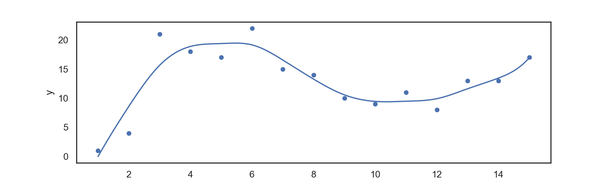
The first method available here is a regression spline. We split the data along the time axis into $k$ interior knots, and fit a piecewise polynomial between each knot. Additionally, we enforce smoothness constraints such that each successive polynomial has continuous value, first, and second derivatives at each knot point where it meets. We use two different basis construction methods here --- BSplines and Power Basis splines.

Power Basis

The power basis representation of a spline is found by augmenting the basis for a polynomial regression problem of that same order with additional basis functions at each knot; this is done to enforce our continuity constraints.

For some degree $n$ basis with $k$ knots, our basis representation is given by:

$$\begin{array}{lll} b_{1}(x)=1, & b_{2}(x)=x, & b_{3}(x)=x^{2}, [...], & b_{n}(x) = x^n \\ \end{array}$$

$$\begin{array}{lll} b_{n+1}(x) = \left(x-k_{1} \right){+}^{n} , & b{n+2}(x) = \left(x-k_{2} \right)_{+}^{n}, [...] \ \end{array}$$

$$\begin{array}{lll} b_{n+k}(x) = \left(x-k_{k} \right)_{+}^{n} \\ \end{array}$$

Where $(x)_+$ is zero if $x$ is negative, and $x$ otherwise.

For data in 'input.csv', we can return a power basis regression spline with:

./splines PowerBasis power knots

for example,

./splines PowerBasis 3 2

Returns a regression spline with degree $3$ with $2$ knots. The output is given as time series data in 'output.csv'. Example output for the above code is given by:

t	y
1	-0.947246
1.1	0.320104
1.2	1.53814
1.3	2.70769
...	...

Which can be automatically plotted with the attached plotting.py file, returning:

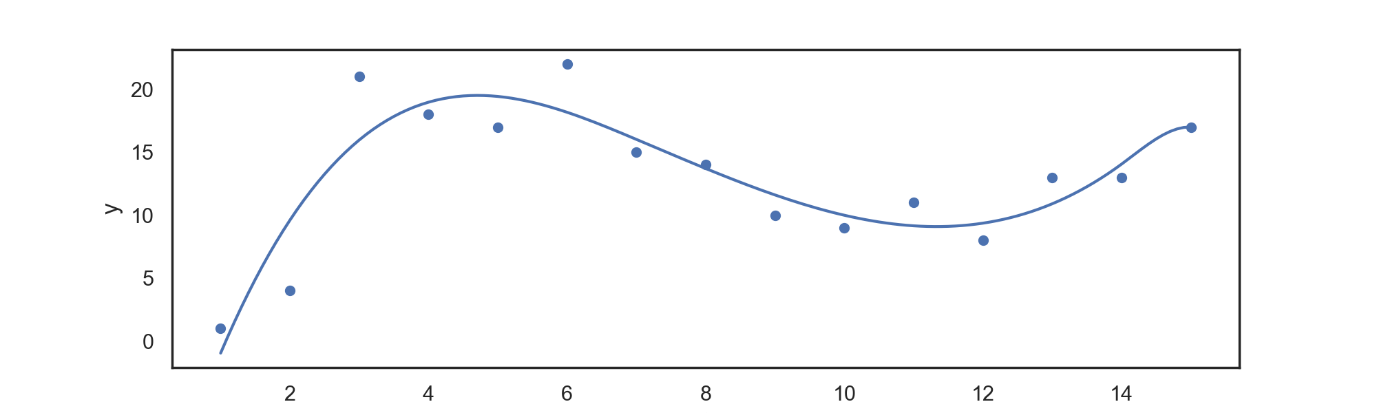
(using the default input.csv provided as data).

Notes:

• Asking for more knots than datapoints probably won't work, for nearly all regression problems. The program will throw a warning when fitting, and let you know if something went wrong.

• Larger computations should use B-Splines instead.

B-Splines

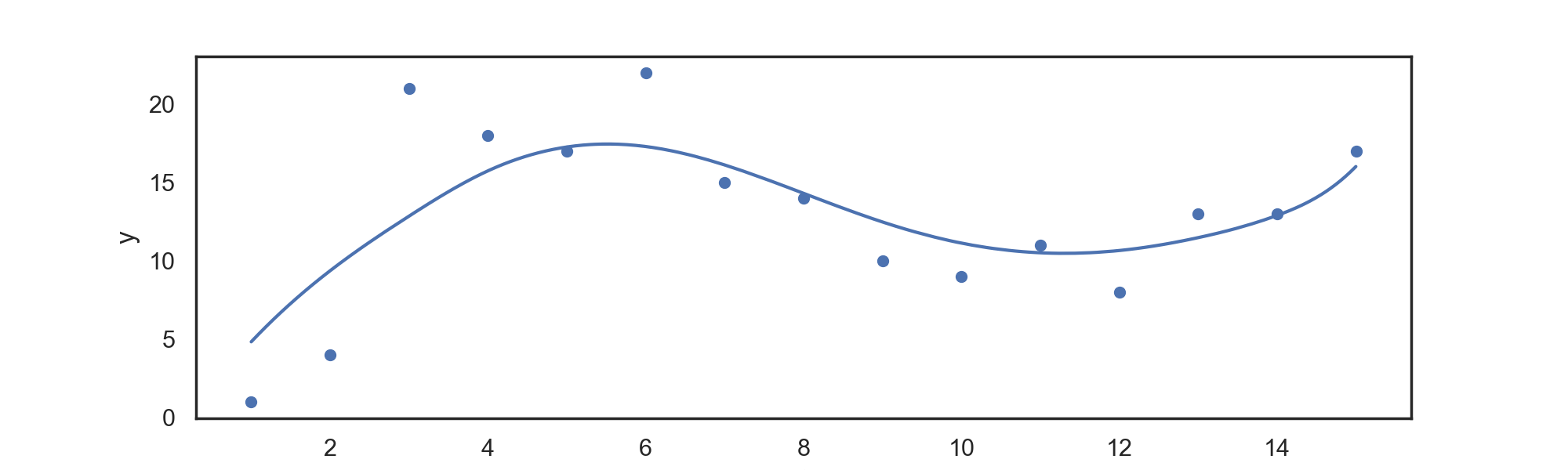
Although computationally simple, the power basis provided above has numerous undesirable numerical properties --- specifically, it requires the computation of large numbers, which can lead to rounding problems. To solve this issue, we turn towards an alternative basis construction which can span the same set of functions as a clamped power basis, but which has more desirable numerical properties.

Another advantage to Basis splines is that they are zero for all values far away from knots points, providing local support. This helps avoiding colinearity issues common with other basis representations.

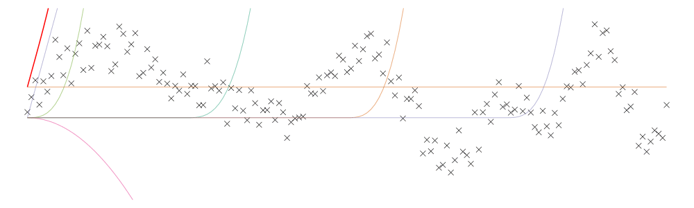
Unlike the power basis, higher order B-spline basis functions have no simple closed form, and must be represented as the iterative convolution of lower order basis functions, where the $0$-th order is an indicator function on successive knots.

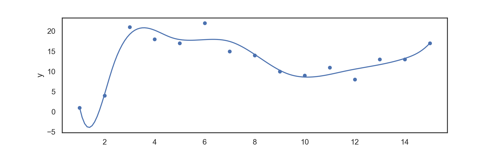
For data in 'input.csv', we can return a power B-spline regression spline with:

./splines BSpline power knots

for example,

./splines BSpline 3 6

Returns a regression spline with degree $3$ with $6$ interior knots. The output is given as time series data in 'output.csv'. Example output for the above code is given by:

t	y
1	0.993459
1.1	-1.38922
1.2	-2.93915
1.3	-3.74152
...	...

Which can be automatically plotted with the attached plotting.py file, returning:

Polynomial Regression

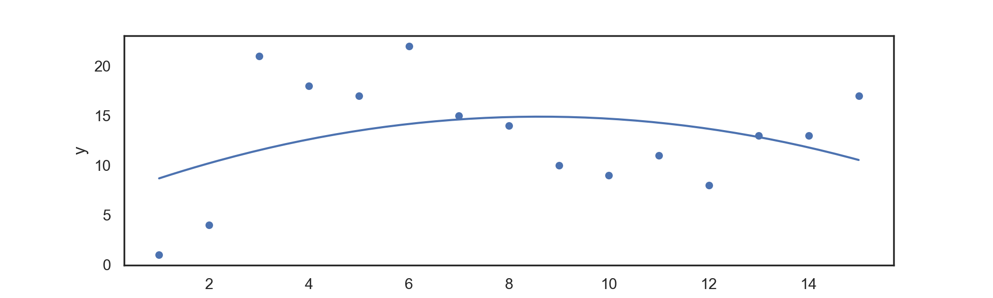
This program can also perform simple polynomial regression, for testing purposes.

For data in 'input.csv', we can return a polynomial regression fit with:

./splines PolynomialRegression power

For example:

./splines PolynomialRegression 2

For a quadratic regression fit, which can be automatically plotted with the included script, returning:

Smoothing Splines

Seeking to avoid questionable heuristics around automatic knot number and location, we assign the maximal number of knots (equal to number of data points), and then penalize the parameters on each individual basis function during fitting. Keeping with tradition, we penalize wigglyness, given by:

$$\lambda \int f^{\prime \prime}(x)^{2} d x$$

for basis function $f$.

For data in 'input.csv', we can return a B-spline smooth with:

./splines Smooth lambda

for example,

./splines Smooth 0.4

Returns a smooth with wiggliness parameter lambda.

t	y
1	-0.00671362
1.1	1,0.920172
1.2	1.82914
1.3	2.72146
...	...

Which can be automatically plotted with the attached plotting.py file, returning:

Automatic Determination of Lambda

Our main concern in this case is one of overfitting — to avoid this, we need to choose lambda such that our model is not overly smooth (maximal bias), and not overly sensitive to individual data (maximal variance).

Attempt to select lambda by hand can work, but ideally we'd like some sort of automatic criteria to select lambda such that we avoid overfitting on the data.

The standard approach is to use some sort of cross validation, portioning the data into different train and test sets to evaluate generalization error.

Here we use Leave One Out cross validation, fitting the data to everything except for one data point, and then testing our performance on that one datapoint, iterating over all the data. That is, for $\hat f^{[-1]}_i $ — the model fit to all data except $y_i$ — we calculate:

$$\mathcal{V}{o}=\frac{1}{n} \sum{i=1}^{n}\left(\hat{f}{i}^{[-i]}-y{i}\right)^{2}$$

(Wood 2006), seeking to select lambda such that we minimize $V_0$. Refitting the model for $n$ datapoints would be computationally intensive. To avoid this, Wood shows:

$$\mathcal{V}{o}=\frac{1}{n} \sum{i=1}^{n}\left(y_{i}-\hat{f}{i}\right)^{2} /\left(1-A{i i}\right)^{2}$$

Deriving the general cross validation score:

$$\mathcal{V}{g}=\frac{n \sum{i=1}^{n}\left(y_{i}-\hat{f}_{i}\right)^{2}}{[n-\operatorname{tr}(\mathbf{A})]^{2}}$$

Where $A$ is the influence matrix and $\hat f$ is the estimate from fitting all the data.

Note: Although this is computationally much cheaper than calculating a new smooth for each datapoint, this is still extremely costly, and can take a while computationally.

To use this method, request 'auto' as the lambda parameter, e.g.

./splines Smooth auto

Returns a smooth with automatically determined wiggliness parameter.

Algorithms Used

Non-trivial algorithms (e.g., anything more complicated than constructing a Vandermonde matrix:)

Cox De Boor Recurrence

Setting a base case as the degree zero basis function — given by an indicator function between knots — we evaluate:

$$B_{i, p}(x)=\frac{x-k_{i}}{k_{i+p}-k_{i}} B_{i, p-1}(x)+\frac{k_{i+p+1}-x}{k_{i+p+1}-k_{i+1}} B_{i+1, p-1}(x)$$

For:

• Knots $t_m$
• Real number $x$
• Basis of degree $p$

Where each $B_{m, p-1}$ is a recursive function call.

GCV

Seeking to avoid calculating new scores for each point in a leave-one-out cross validation test, we employ a clever trick, fitting the model once per $\lambda$ value, and then evaluating:

$$\mathcal{V}{g}=\frac{n \sum{i=1}^{n}\left(y_{i}-\hat{f}_{i}\right)^{2}}{[n-\operatorname{tr}(\mathbf{A})]^{2}}$$

Where

• $y_i$ is the dropped point.
• $\hat f_i$ is the function evaluated at that point.
  • This is essentially the Sum of Squared Errors.
• Divide out by the number of points minus the trace of the Hat Matrix.
  • The hat matrix is a [data, data] sized matrix that produces the model fits when multiplied by the predictor variables.
  • Given by $\mathbf{X}\left(\mathbf{X}^{\top} \mathbf{X}+\lambda \mathbf{S}\right)^{-1} \mathbf{X}^{\top}$

Gaussian Elimination

With one exception, systems are solved in this package via Gaussian elimination (instead of calculation of the inverse), and then back substitution. This algorithm is not the focus of the project, but it plays a key role, so a description here seems useful.

• The goal is to solve a system of type "X \ y" in Matlab / Julia notation.
• Augment X with vector y on the right hand side.
• Loop over all the columns
  • Loop over all the rows
    • For any value below a pivot, calculate the new value required such that subtracting the multiple of this value times the pivot from the target row will make the original value zero.
    • Add a the pivot row multiplied by this value to that entire row.
    • Repeat until the matrix is upper triangular.
• Starting with the last element of the lower triangular matrix, construct the solution vector by iterating up over the rows of the matrix.

Due to the matrix inverse being ill-conditioned, this is vastly preferable to explicit computations of $\hat \beta$. Unfortunately, when calculating the hat matrix, an inverse needed to be computed exactly. Ideally an alternative should be implemented here, using some sort of decomposition (e.g. SVD) to recover a more well conditioned estimate.

In the case of an explicit inverse, the above algorithm was modified slightly:

• Augment with an identity matrix.
• Eliminating all off-diagonal elements.
• Set pivots to zero.
• Return resultant transform of identity as matrix inverse.

This is far from ideal, but for the crude computation of GCV that it is used for, it doesn't totally vitiate the project.