Equispaced data with gaps vs Non-equispaced data

[wgprojects]

Can anyone help clear up my misunderstanding?

I used the forward transform to convert a sine wave to frequency domain, then adjoint transform to go back to time domain.
If the data is equispaced, this works well (not pictured).

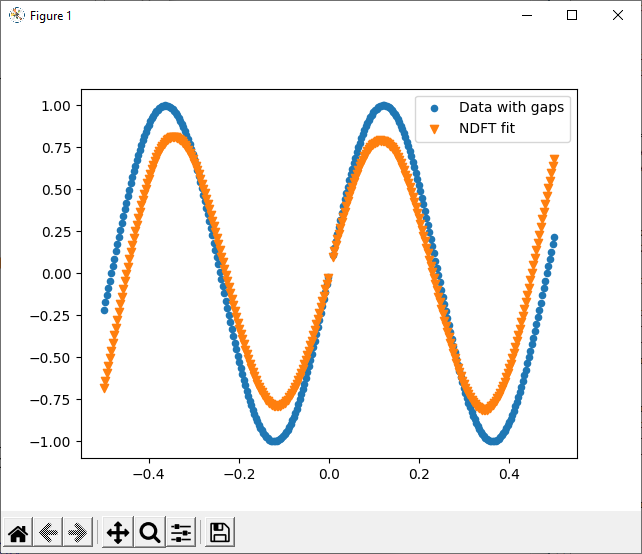
If the data is equispaced but with even a small gap (<1% missing) the reconstruction is smooth, but with incorrect amplitude:

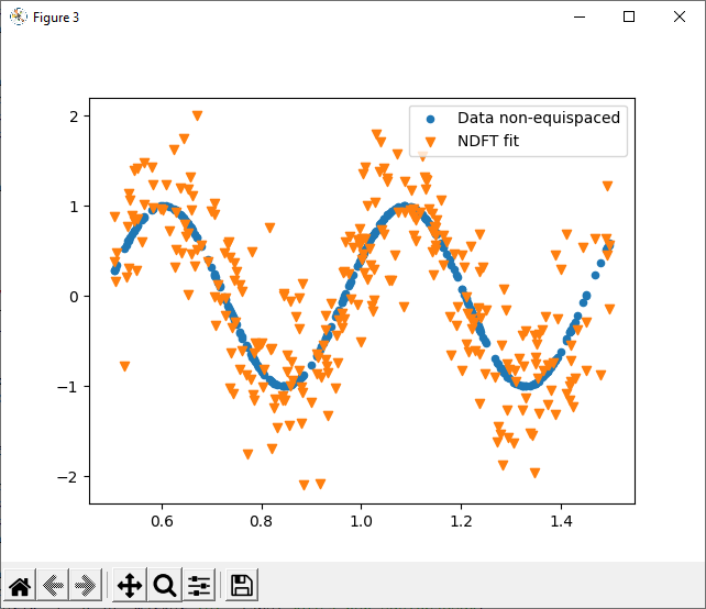
If the data is non-equispaced, the reconstruction is very poor. The Fourier coefficients appear totally random - not an ideal spike, and not spectral leakage.

Is this technique not intended for just these applications? I believe it is and that I've made a mistake.

`import nfft
import numpy as np
import matplotlib.pyplot as plt

freq = 13 #Rad/s
N = 300

x = np.linspace(-0.5, +0.5, N)
f = np.sin(freq*x)

#Equally spaced data with one gap:

gapsize = 2
x=np.delete(x, slice(N//2,N//2+gapsize), axis=0)
f=np.delete(f, slice(N//2,N//2+gapsize), axis=0)

N = len(x)
k = -N//2 + np.arange(N)

f_k = nfft.ndft(x, f)

plt.figure(2)
plt.scatter(k, f_k.real, label="Real")
plt.scatter(k, f_k.imag, label="Imag")
plt.legend()

f_hat = nfft.ndft_adjoint(x, f_k, N)/N
plt.figure(1)
plt.scatter(x, f, s=20, marker='o', label="Data with gaps")
plt.scatter(x, f_hat, s=35, marker='v', label="NDFT fit")

plt.legend()

#Randomly spaced data
x = 0.5 + np.random.rand(N)
f = np.sin(freq*x)

N = len(x)
k = -N//2 + np.arange(N)

f_k = nfft.ndft(x, f)

plt.figure(4)
plt.scatter(k, f_k.real, label="Real")
plt.scatter(k, f_k.imag, label="Imag")
plt.legend()

f_hat = nfft.ndft_adjoint(x, f_k, N)/N
plt.figure(3)
plt.scatter(x, f, s=20, marker='o', label="Data non-equispaced")
plt.scatter(x, f_hat, s=35, marker='v', label="NDFT fit")

plt.legend()
plt.show()
`

[Peter Neigel]

It seems like ndft_adjoint is actually the function to go from signal into frequency space, and ndft to go from frequency into signal space.

freq = 3
N_samples = 500

x = np.linspace(0, 1, N_samples) # 1 is arbitrary here. This is the time range of your data
f = np.sin(freq*2*np.pi*x)

# Equally spaced data

plt.scatter(x,f)
plt.title("Equally spaced signal")
plt.show()

N_freq = 100
k = -N_freq//2 + np.arange(N_freq)

f_k = nfft.ndft_adjoint(x, f, N_freq)

plt.figure(2)
plt.plot(k, np.abs(f_k), label="Absolute")
plt.legend()
plt.title("Frequency spectrum for equally spaced signal")
plt.show()

print("Maximum at ", k[np.argmax(np.abs(f_k))])

f_hat = nfft.ndft(x, f_k)/N_samples
plt.figure(1)
plt.scatter(x, f, s=35, marker='o', label="Data with gaps")
plt.scatter(x, f_hat, s=15, marker='v', label="NDFT fit")
plt.legend()
plt.title("Reconstruction for equally spaced signal")
plt.show()

#Equally spaced data with one gap:

gapsize = 30
x=np.delete(x, slice(N_samples//2,N_samples//2+gapsize), axis=0)
f=np.delete(f, slice(N_samples//2,N_samples//2+gapsize), axis=0)

N_freq = 100
k = -N_freq//2 + np.arange(N_freq)

f_k = nfft.ndft_adjoint(x, f, N_freq)

plt.figure(2)
plt.plot(k, np.abs(f_k), label="Absolute")
plt.legend()
plt.title("Frequency spectrum for equally spaced signal with gap")
plt.show()

print("Maximum at ", k[np.argmax(np.abs(f_k))])

f_hat = nfft.ndft(x, f_k)/(N_samples-gapsize)
plt.figure(1)
plt.scatter(x, f, s=35, marker='o', label="Data with gaps")
plt.scatter(x, f_hat, s=15, marker='v', label="NDFT fit")
plt.legend()
plt.title("Reconstruction for equally spaced signal with gap")
plt.show()

#Randomly spaced data
x = np.random.rand(N_samples)
f = np.sin(freq*2*np.pi*x)

N = len(x)
k = -N_freq//2 + np.arange(N_freq)

f_k = nfft.ndft_adjoint(x, f, N_freq)

plt.figure(4)
plt.plot(k, np.abs(f_k), label="Absolute")
plt.title("Frequency spectrum for randomly spaced signal")
plt.legend()
plt.show()

print("Maximum at ", k[np.argmax(np.abs(f_k))])

f_hat = nfft.ndft(x, f_k)/N_samples
plt.figure(3)
plt.scatter(x, f, s=20, marker='o', label="Data non-equispaced")
plt.scatter(x, f_hat, s=35, marker='v', label="NDFT fit")
plt.title("Reconstruction for randomly spaced signal")
plt.legend()
plt.show()

result: