- Introduction
- Data description
- Data visualization
- Data preprocessing
- Data cleaning
- Model selection
- Metrics choice
- Loss function choice
- Optimizer choice
- Data representation
- Implementation strategy (PyTorch)
- Initial guesses
- Model training
- Model testing
- Improvements
- Project files' description
- Short models' reference
- About author
- References
The task is given by WINSTARS.AI company. It states:
The goal of the test project is to build a semantic segmentation model. Prefered tools and notes: tf.keras, Unet architecture for neural network, dice score, python.
Results of your work should contain next:
- link to GitHub repository with all source codes;
- code for model training and model inference should be separated into different .py files;
- readme.md file with complete description of solution;
- requirements.txt with required python modules;
- jupyter notebook with exploratory data analysis of the dataset;
- any other things used during the working with task;
Source code should be well readable and commented;
Project has to be easy to deploy for testing.
The objective of the project is to build a semantic segmentation model using Python, optionally including the suggested technologies, while maximizing Dice and separating different project modules into different files.
The problem being researched is a Kaggle competition with a vast amount of images. The decision of using the Kaggle environment was made due to its simplicity, convenience and speed (at the time of selection).
We are limited in terms of GPU by 30 hours per week by the Kaggle platform. Additionally, the system tends to terminate long-run sessions (multiple-epoch trainings) or freezes when the tab is inactive. It restrics the RAM usage as well, meaning the high resolution images or large batch sizes would not be able to be processed either.
The most popular frameworks for Data Science and Machine Learning are the two prominent options: TensorFlow and PyTorch. While both frameworks continue to evolve, each possesses its own set of advantages and disadvantages.
Having had an experience in both frameworks while learning, Tensorflow has often encountered challenges in ensuring reproducibility (at least on CUDA). Additionally, implementing changes at various stages proved to be harder to implement, less intuitive and user-friendly compared to PyTorch's.
It is considered, however, that Tensorflow fits production and scalable projects more; moreover, it is preferred for models' deployment on mobile devices and has a larger community due to being older than PyTorch.
On the contrary, PyTorch is more suitable for flexibility and research, utilizing the same functionality within multiple projects and have a complete reproducability, which is crucial for any Machine Learning project (for instance when determining a single augmentation to be applied, we would need to perform only one training). There is also a plethora of native features that PyTorch provides and Tensorflow doesn't: various loss functions, optimizers with complicated set-ups and metrics, data loaders and custom samplers within their native OOP mechanics.
Given the preference for exploring new ideas and ensuring reproducibility on GPU; being a student, researcher, constantly trying new ideas, I have given my preference to PyTorch. (Tensorflow does have reproducability on Cuda in the experimental module, but it leads to slowing the process down and makes it indiscernible from CPU operations in terms of model training, making it meaningless to utilize parallel evaluations as such).
P.S.: My perception is limited and biased, I was taught this way and inherited not only knowledge, but the spirit of my teacher whom I sincerely adore. However, I have tried implementing the project utilizing Tensorflow and Keras first and gave up after I lost control of the reproducability having switched to GPU. Training results in Tensorflow were also worse (I assume the scores were a matter of my mistakes).
All of the instruments used are popular and well-known. I suggest we look at them as a code for convenience:
import os                       # interacting with the operating system
import sys                      # interacting with the Python interpreter
import pandas as pd             # For data manipulation and analysis
import numpy as np              # For numerical computing
import gc                       # For garbage collection
import random                   # For generating random numbers

import cv2                      # For computer vision tasks
from PIL import Image           # For image processing
import albumentations as albu   # For image augmentation

import matplotlib.pyplot as plt # For plotting
from sklearn.model_selection import train_test_split  # For splitting data into train and test sets

import torch                    # PyTorch library
import torch.nn as nn           # PyTorch's neural network module
import torch.optim as optim     # For optimization algorithms
from segmentation_models_pytorch import utils  # Utilities for segmentation models
import segmentation_models_pytorch as smp  # PyTorch segmentation models
from torch.utils.data import Dataset, DataLoader  # For creating custom datasets and data loaders
from tqdm import tqdm  # For displaying progress bars during loops
Seen above libraries can be separated into 4 groups:
- frequently-used Python modules of general usage
- working with images (including plotting and augmenting)
- plotting and separating data
- a regular set of
PyTorchmodules
The data is a set of ship images taken from a satellite. They are represented via a .csv file and the respective images. Its columns are:
- ImageId - represents the name of the image with the
.jpgextension - EncodedPixels - RLE encoded mask for the respective image
- Ships (custom) - how many ships is present on the image
- Size_kb (custom) - image size in kb
Before proceeding to working with the dataset, we should look at it and obtain some basic information. Issues having been addressed:
Taking the first image for an initial guess, we check if others have the same dimensions. It is confirmed that all images are indeed (768, 768).
Each first number in the mask represents the pixel number and each second - the quantity of filled pixels after. A custom function was implemented according to the above explanation.
We can look at the problem as:
- a ratio of single-ship images to numerous-ship images
- a ratio of non-ship images to images with ships.
Both hypothesis were addressed empirically (simple and improved models respectively).
By printing unique ImageIds within the dataframe, the observation has proved that a significant part of ids is repeated. That is because the mask describes only one ship per line in the .csv, so the images were grouped, concatenating masks accordingly.
As representations of an empty mask is a plain 0, we have replaced Nans with the latter.
The problem: corrupted / invalid / error-read / out-of-topic images.
A complex problem. I have inspected images within my file system and noticed that sometimes they are exclusively clouds, lands or simply noise (blue squares). I have sorted them out by image size and, emperically, most of them were in the files of less or equal to 52 kb.
With nearly 200 000 images, manually inspecting each picture is not feasible. We would need to use other classifying algorithms for that presumably. Despite of that, I came across a solution by a researcher on Kaggle (ABNERZHANG), who had previously dealt with the problem and provided his results on the platform for everyone. It would be a shame not to have respected his efforts.
The suggested Unet model is indeed popular and suitable for this type of tasks. It similarly aligns with the limitations listed by the number of trainable parameters (depending on the specific architecture).
The IoU is often utilized due to its ease of understanding to a human eye in terms of assessing a model's performance. Nonetheless, the suggested Dice is an option with a higher ephasis on intersection, rather than both intersection and difference equally, as with IoU. Given the serious class imbalance problem, where it is critical to identify objects and avoid mistakes, Dice would give higher scores here, so the metric is indeed suits better. Thus, Dice it is.
As we are dealing with the task of maximizing Dice, we want to make sure to minimize the Dice error loss. It was picked as a "counterforce" to maximize the metric. So it is the first on the list. However, it is always "a matter of model complexity and data combination", so we will try all commonly used loss functions for the current scenario:
- Focal loss - Cross Entropy based loss function; designed to address class imbalance and focuses on hard examples during training (matches our case accurately)
- Lovasz loss - suits binary problem; designed to optimize for the intersection over union (
IoU) metric (unlikely to work as our metric isDice) - Binary Cross Entropy with Logits Loss - Cross Entropy based; suits binary problem; designed for binary classification tasks
Adam, as a state-of-art optimizer, fits almost in any case: adaptive learning rate, efficiency, low memory requirements, ease of use. These are on the list unless they are needed:
Adam- SGD
- RMSProp
- Adagrad
- modifications of aboves
A single item within the dataset is represented as follows:
- Encoded RGB image (batch size, color channel=
3, width, height) - Decoded grayscale mask (batch size, color channel=
1, width, height)
The image is represented as a 3 color channel array [0; 255]. The mask, which is single-channeled, is either 0 (for an empty mask, i.e. no ships on the image) or an image-sized array filled with 0 and 1, where 0 represents a non-ship pixel, 1 - a ship pixel.
We will have a custom class for training, visualization and debugging the model called TrainAndTestModel. Mostly used are its methods train and continue_training, names of which speak for themselves. The second one can be utilized if the training is terminated in any moment without the necessity of starting over.
For these we will have to create a DataLoader that creates batches of data.
And for the DataLoader to work, we will need a custom dataset class that I have titled AirbusShipDetectionDataset, specifically its __getitem__ method that will be utilized by the DataLoader. It represents a single item of a dataset.
Besides that, we have an additional task to address - class imbalance, according to which the decision to create a custom sampler has been made. It is utilized by the DataLoader and called ShipStratifiedSampler. Due to the strong class imbalance, I have undersampled images with no ships, but don't have enough certainty that it will help the model. That is why I have created a sampler that takes a tunable parameter zero_ships_ratio_per_batch for the ratio of empty images per batch. It would answer this question once and for all.
It tends to be low for segmentation problems, but still varies from case to case, so 1e-4 is chosen as an initial guess.
Depends on data complexity. It is mostly 5 in the project for a representative plot while tuning the model. Later, we run more epochs, often 5 each time so that we can detect an overfit earlier and save the best state of the model.
A good practice is to pick odd numbers to avoid patterns/seasonalities (this is not the case here). Adjusted to 16 during experimentation due to a slight overfit.
Segmentation tasks often utilizes the ReduceLROnPlateau to fine-tune the model, when the score at its peak and we are looking for a better-fit local minimum with extremely small (and/or different) steps to avoid overshooting and get a better understanding of the surface area of the function we're minimizing. For time-saving purposes it was also applied at the end.
Due to the Kaggle's restrictions, images being researched were downscaled to (256,256).
They are applied as a matter of regularization for the model in case of overfit or to provide more diversity to an existing dataset by altering the appearance of some images. Initially (and later on), the following augmentations are used:
albu.Compose([
    albu.Resize(*INPUT_SIZE),   # resize to (256,256)
    albu.Normalize(),           # normalizes the dataset according to the imagenet's mean and std
])A popular resnet18 Unet modification is chosen and its complexity has been researched. It may be simplified / complexed in 2nd or 3rd modification.
The very first parameter we want to get along with. I have considered undersampling of non-ship images. Firstly, we research the impact of the amount of non-ship images on the model's performance. Initial guess is 0.25 per batch of 16:
$ 16 * 0.25 = 4 $ images.
The best Dice:Loss here is 0.474:0.989. Looking at the ZERO_SHIPS_RATIO_PER_BATCH decreasing, we start to see the increase in metrics:
| ZERO_SHIPS_RATIO_PER_BATCH | Dice | Loss |
|---|---|---|
| 0.25 | 0.474 | 0.989 |
| 0.15 | 0.490 | 0.987 |
| 0.10 | 0.537 | 0.986 |
| 0.00 | 0.539 | 0.985 |
The best model's performance; plotted:

The optimal value ZERO_SHIPS_RATIO_PER_BATCH= 0.0.
The next issue to address is an issue of a high loss. Proceeding to try different losses:
| Loss function | Dice | Loss |
|---|---|---|
| Dice loss | 0.539 | 0.985 |
| Focal loss | 0.759 | 0.172 |
| Lovasz loss | 0.001 | 1.000 |
| BCEWithLogits loss | 0.821 | 0.691 |
Both Focal and BCEWithLogits losses look well, but based on the metric being optimized, the one with the lower loss is chosen.
The best model's performance; plotted:

The plot looks stunning to me, the learning rate remained untouched (1e-4).
The batch size of 16 seems to be perfectly in tact with the model's complexity and the learning rate. To make sure we have the best possible performance at this stage, the batch size has been researched too:
| Batch size | Dice | Loss |
|---|---|---|
| 9 | 0.762 | 0.172 |
| 16 | 0.759 | 0.172 |
| 25 | 0.739 | 0.172 |
The batch size remained untouched due to the fact that a batch size of 9 creates more batches, consumes more time and according to the plot, overfits early:
It is hard to imagine a computer vision task without augmentations. The list of tried augmentations and their combinations:
albu.RandomRotate90(p=0.5),
albu.HorizontalFlip(p=0.5),
albu.VerticalFlip(p=0.5),
albu.ShiftScaleRotate(shift_limit=0.1, scale_limit=0.2, rotate_limit=45, p=0.5),
albu.RandomBrightnessContrast(p=0.5),
albu.GaussianBlur(blur_limit=(3, 5), p=.5),
albu.ElasticTransform(p=0.5, alpha=120, sigma=120 * 0.05, alpha_affine=120 * 0.03),
albu.GaussNoise(var_limit=(10.0, 20.0), p=.5),
albu.Cutout(num_holes=1, max_h_size=16, max_w_size=16, p=.5),
albu.ColorJitter(brightness=0.1, contrast=0.1, saturation=0.1, hue=0.2, p=.5),
albu.GridDistortion(p=0.5),
albu.OpticalDistortion(distort_limit=0.5, shift_limit=0.5, p=0.5),
None of them or their combinations has worked. I presume the conclusion behind this is the data's being wholesome and diverse. It combines beautifully with the model's complexity. This is also the reason why we don't consider simplifying or complexing the resnet18 to anything else.
It is high time we maximized the score having tuned the parameters. I have summarized the trainings performed:
| Model 1 (part 1) | ||||
|---|---|---|---|---|
| learning rate | 1e-4 | 1e-5 | 1e-5 | 1e-10 |
| batch size | 16 | 16 | 16 | 16 |
| epochs | 5 | 5 | 5 | 1 |
| augs | norm + reshape | norm + reshape | norm + reshape | norm + reshape |
| optim | Adam | Adam | Adam | Adam |
| dice | 0.75926 | 0.81629 | 0.83660 | 0.841535 |
| loss | 0.17284 | 0.17279 | 0.17277 | 0.172753 |
| shape | 256x256 | 256x256 | 256x256 | 256x256 |
| scheduler | - | redLROnPlat(max,0.1,1) | redLROnPlat(max,0.1,1) | redLROnPlat(max,0.1,1) |
| Model 1 (part 2) | ||||
|---|---|---|---|---|
| learning rate | 1e-10 | 1e-10 | 1e-10 | 1e-10 |
| batch size | 16 | 16 | 16 | 16 |
| epochs | 1 | 1 | 1 | 1 |
| augs | norm + reshape | norm + reshape | norm + reshape | norm + reshape |
| optim | Adam | Adam | Adam | Adam |
| dice | 0.841536 | 0.841536 | 0.841536 | 0.841536 |
| loss | 0.172753 | 0.172753 | 0.172753 | 0.172753 |
| shape | 256x256 | 256x256 | 256x256 | 256x256 |
| scheduler | redLROnPlat(max,0.1,1) | redLROnPlat(max,0.1,1) | redLROnPlat(max,0.1,1) | redLROnPlat(max,0.1,1) |
| Model 1 (part 3) | |||||
|---|---|---|---|---|---|
| learning rate | 1e-9 | 1e-8 | 1e-7 | 1e-8 | 1e-9 |
| batch size | 16 | 16 | 16 | 16 | 16 |
| epochs | 1 | 1 | 2 | 1 | 1 |
| augs | norm + reshape | norm + reshape | norm + reshape | norm + reshape | norm+reshape |
| optim | Adam | Adam | Adam | Adam | Adam |
| dice | 0.841539 | 0.841661 | 0.84222 | 0.84252 | 0.84251 |
| loss | 0.172753 | 0.172753 | 0.17274 | 0.17275 | 0.17275 |
| shape | 256x256 | 256x256 | 256x256 | 256x256 | 256x256 |
| scheduler | redLROnPlat(max,0.1,1) | redLROnPlat(max,0.1,1) | redLROnPlat(max,0.1,1) | redLROnPlat(max,0.1,1) | redLROnPlat(max,0.1,1) |
The best Dice:Loss combination is 0.84251:0.17275:

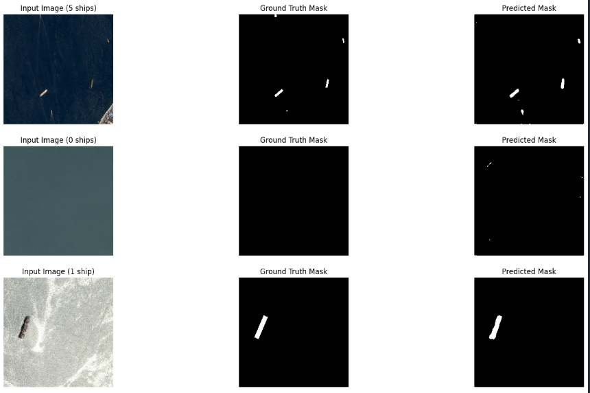
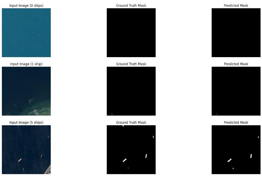
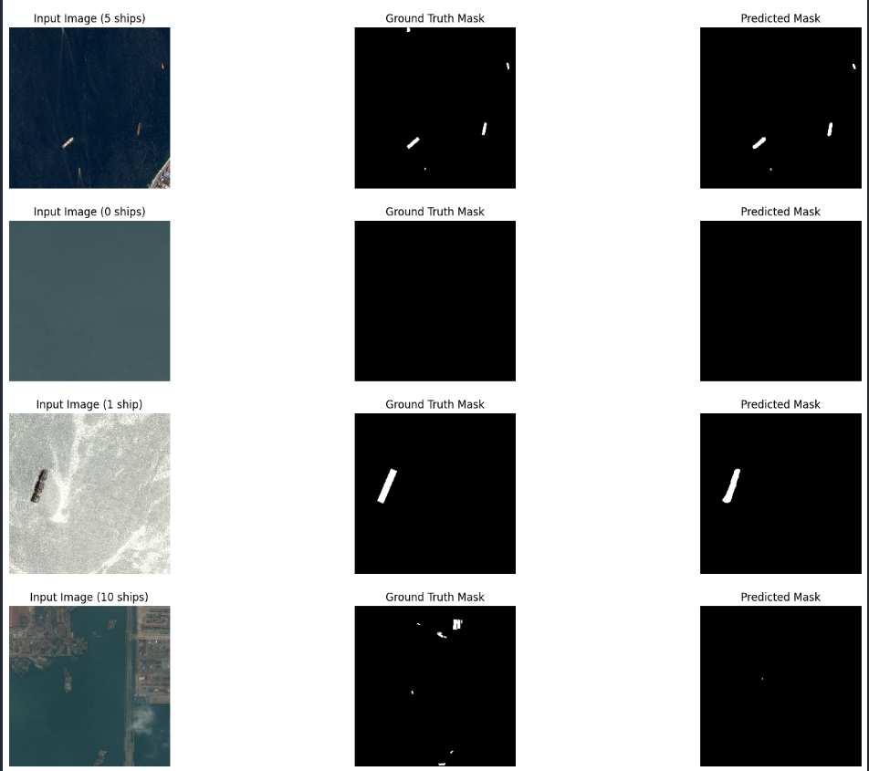
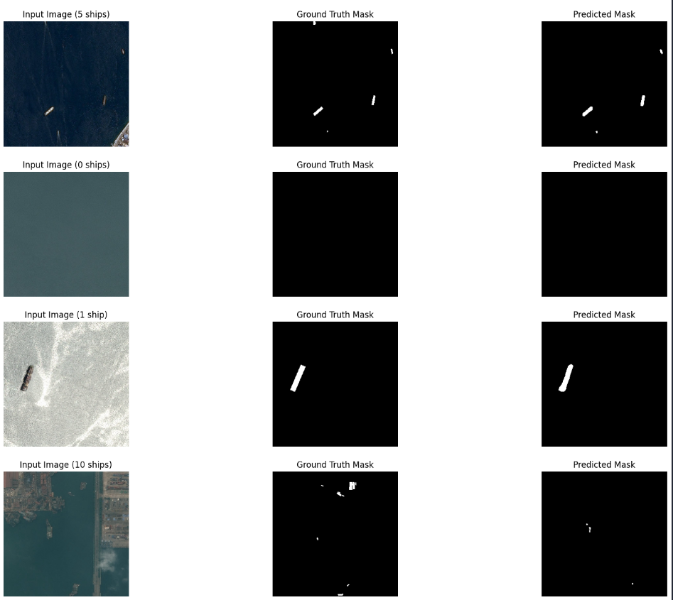
For the testing, I have picked 9 unseen images (from the validation data) and divided them into 3 groups: no-ship images, single-ship images and multiple-ship images.
The model has shown its best performance with the threshold of 1e-2, but has problems with identifying multiple ships. The model with lower thresholds results in a lot of noise in simpler cases while doing better fixating multiple ships (the trade-off is not worthy).
- The model has no problem identifying that an image has no ships on it. No wonder that the
ZERO_SHIPS_RATIO_PER_BATCHwas the best at its value of0. - The value of
THRESHOLD=1e-2is an optimal choice. Values below it will result in noise (false positives) on pictures with fewer or no ships, above it - in bad-quality multiple ships predictions (it "thinks" there are fewer). The model is struggling with numerous ships.
Thinking of how numerous ships are the problem, I have come up with a solution of stratification by the amount of ships. The class of the custom sampler was changed to ShipStratifiedSampler and now takes a multiple_ships_ratio_per_batch parameter that is responsible for a multiple ships amount per batch.
During the training, most of the latter training structure was preserved and the multiple_ships_ratio_per_batch coefficient was evaluated as follows:
$ 21445 + 12217 = 33662 $ images for training
$ 33662 // 16 = 2103 $ batches
Having $ 21445 // (16 * (1 - x)), $ solve x ->
$ x = 0.3629 $ to avoid samples` repetition as much.
The best Dice:Loss pair was 0.84761:0.17276.
The option of 4e-4 has appeared to be the most optimal.
The second model results in identifying multiple ships more accurately, but more biased towards fewer-ship predictions. I have intentionally picked a slightly more overfit version (in terms of epochs) to address the issue of noise.
I have summarized the trainings performed:
| Model 2 (part 1) | ||||
|---|---|---|---|---|
| learning rate | 1e-4 | 1e-5 | 1e-5 | 1e-10 |
| batch size | 16 | 16 | 16 | 16 |
| epochs | 5 | 5 | 5 | 5 |
| augs | norm + reshape | norm + reshape | norm + reshape | norm + reshape |
| optim | Adam | Adam | Adam | Adam |
| dice | 0.77497 | 0.82578 | 0.84657 | 0.84761 |
| loss | 0.17282 | 0.17277 | 0.17276 | 0.17276 |
| shape | 256x256 | 256x256 | 256x256 | 256x256 |
| scheduler | - | redLROnPlat(max,0.1,1) | redLROnPlat(max,0.1,1) | redLROnPlat(max,0.1,1) |
| Model 2 (part 2) | |
|---|---|
| learning rate | 1e-10 |
| batch size | 16 |
| epochs | 5 |
| augs | norm + reshape |
| optim | Adam |
| dice | 0.84761 |
| loss | 0.17276 |
| shape | 256x256 |
| scheduler | redLROnPlat(max,0.1,1) |
As the model is struggling identifying numerous ships we can apply augmentations to only those and combine it with the first modification. Therefore, we may implement two more tunable parameters: multiple_ships_ratio_per_batch=0.3629 for controlling how many multiple-ship images will be per batch (no reason to pick less as we are decreasing the amount of training data; same risky to go further as we might overfit the model) and ships_threshold_for_add_augs for the amount of ships that should take additional augmentations.
As an option we could refuse of stratification completely as in the first modification and only try to adjust the ships_threshold_for_add_augs.
As the modifications mentioned above are not within the scope of the project, they are left to the observer as a puzzle. As a matter of interest, I have tried to apply a few and it seems to me upon first inspection, that whenever the dice goes up, the loss goes up; whenever the dice goes down, the loss goes down. It is a problem of the trade-off of what we want to achieve. We may want to be extremely precise or avoid mistakes more. To hold both simultaneously, we could consider simplifying/complexing the model and tuning it again.
As the task has required to maximize Dice, the second model is chosen as a superior one and will be presented in the training file of the final project. Its training takes less time and code and it is more prune to the class imbalance problem.
- README.md - complete description of solution
- src - directory with images for the README.md
- requirements.txt - required python modules
- notebook.ipynb - initial notebook containing EDA + training + testing + developing + experimenting + thoughts
- EDA.ipynb - exploratory data analysis of the dataset + data preprocessing and cleaning
- train_ship_segmentation_post_EDA.csv - original .csv data representation after the EDA
- training.py - code for the model training (modification 1st)
- inference.py - code for the model inference
- models/model_1_simple_unet_semantic_segmentation.pt - saved model (simple; no modifications)
- models/model_2_sratified_unet_semantic_segmentation - saved model (modification 1st)
| Dice | Loss | Best threshold | Application | |
|---|---|---|---|---|
| Model 1 (simple) | 0.84251 | 0.17275 | 1e-2 | fewer ships |
| Model 2 (stratified by ships) | 0.84761 | 0.17276 | 4e-4 | larger groups+ |
Project by Yurii Dzbanovskyi
- Email: uradzb@ukr.net
- Telegram: +38 096 874 17 18
- https://www.kaggle.com/c/airbus-ship-detection/data
- https://www.kaggle.com/c/airbus-ship-detection/discussion/62921
- https://www.tensorflow.org/api_docs
- https://pytorch.org/docs/stable/index.html
- https://opencv.org/blog/pytorch-vs-tensorflow/#:~:text=Key%20Takeaways,for%20beginners%20and%20rapid%20prototyping.
- https://www.freecodecamp.org/news/pytorch-vs-tensorflow-for-deep-learning-projects/
- keras-team/keras#7937
- keras-team/keras#15586


