Is cigarette smoked per day a factor in determining whether a patient suffers from Coronary Heart Disease? In this analytical study, we can conclude the consistent evidence supporting a causal role of smoking in causing coronary heart disease. Thus establishing a causal relationship between the two.
Every year about 735,000 Americans have a heart attack. Of these, 525,000 are a first heart attack and 210,000 happen in people who have already had a heart attack. About 647,000 people die of heart disease every year–that’s 1 in every 4 deaths. The predicted risk of an individual can be a useful guide for making clinical decisions on the intensity of preventive interventions: such as restrictions on diet, physical activity, drugs. Having a risk stratification approach will be beneficial to settings where saving the greatest number of lives at lowest cost becomes imperative. Coronary artery disease is thought to begin with damage or injury to the inner layer of a coronary artery, sometimes as early as childhood. Theoretically, this damage may be caused by various factors, including:
- Smoking - It is believed, people who smoke cigarettes are at a higher risk of getting coronary heart disease. As a proxy for smoking, we have a variable called ‘cigsPerDay’ which denotes the number of cigarettes a person smokes per day.
- Age - As people get old, the cells in their body start to degenerate. As a result of the degeneration of cells, muscles in the body suffer from muscle atrophy. Heart muscles also undergo muscle atrophy as age increases. We have ‘Age’ that is the age of a person who participated in the study, and this can be used as a potential control variable.
- Gender - A woman’s heart may look just like a man’s, but there are significant differences. For example, a woman’s heart is usually smaller, as are some of its interior chambers. More importantly, Estrogen (a hormone) offers women some protection from heart disease. So as a proxy for gender, we will use ‘Male’ which indicates the gender of the person who participated in the study.
- High blood pressure - Among all heart attack patients, there is one factor that puts them under the radar. That factor is high blood pressure. Nearly any patient who suffered from a heart attack had a history of high blood pressure. As a proxy for high blood pressure, we use ‘BPMeds’ which denotes whether or not a person was on blood pressure medication. If the person is on blood pressure medication, it indicates that he/she has high blood pressure, and thus is at greater risk of coronary heart disease.
- Diabetes or insulin resistance - Insulin resistance occurs when excess glucose in the blood reduces the ability of the cells to absorb and use blood sugar for energy. This is also known as Diabetes. Research shows that the amount of sugar, or glucose, in the blood changes the behavior of blood vessels, making them contract more than normal. This excess pressure makes these blood vessels burst and causes a blood clot, which in turn leads to a heart attack. As a proxy for this, we have ‘glucose’ which indicates the blood sugar level of the person in the study.
- Heart rate - Studies suggest that a persistently high heart rate (or high resting heart rate) is associated with an increase in coronary and cardiovascular death rates, the precise reason for this association remains unclear. It has been attributed to overall lack of physical fitness or poor health. As a proxy for this, we have ‘heartRate’ of people who participated in the study. Abstract The World Health Organization has estimated 12 million deaths occur worldwide, every year due to Heart diseases. Half the deaths in the United States and other developed countries are due to cardiovascular diseases. The early prognosis of cardiovascular diseases can aid in making decisions on lifestyle changes in high risk patients and in turn reduce the complications. This project intends to pinpoint the most relevant/risk factors of developing a coronary heart disease and understand the causal relationship of these factors to answer our business question and hypothesis. In the due course of the completion of this project we have developed a deeper understanding of various concepts of logistic regression and other econometric tools as taught in this course.
Is cigarette smoked per day a factor in determining whether a patient suffers from Coronary Heart Disease? HO : There is no association between Cigarette smoking and risk of CHD.
HA : Cigarette smoking substantially increases the risk of coronary heart disease
-
- Variable of interest: cigarettes smoked per day
- Control Variables: age, male, BPMeds, glucose, heartRate, sysBP, etc.
data = read.csv("framingham.csv")
head(data)
Data has been collected from an ongoing cardiovascular study on residents of the town of Framingham, Massachusetts. The dataset provides the patients’ information. The data has 4238 records, 16 attributes.
- DEMOGRAPHIC *Sex, Age
- BEHAVIORAL
- Current smoker, Cigs per day
- MEDICAL HISTORY
- BP Meds, Prevalent Stroke, Prevalent Hyp, Diabetes
- MEDICAL CURRENT
- Tot Chol, Sys BP, Dia BP, BMI, Heart Rate, Glucose
- TARGET VARIABLE
- TenYearCHD - 10 year risk of coronary heart disease)
There are a NULL Value on education, cigsPerDay, BPMeds, totChol, BMI, heartRate, and glucose feature.
Lets plot the data to see if there are any outliers.
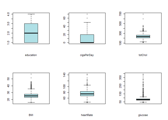
- there is no outlier data on education feature, so we can use mean()
- there are outlier data on cigsPerDay feature, so it should be use median() approach
- on BPMeds author using 0 for the NULL Value.
- there are outlier data on totChol feature, so it should be use median() approach
- there are outlier data on BMI feature, so it should be use median() approach
- there are outlier data on heartRate feature, so it should be use median() approach
- there are outlier data on glucose feature, so it should be use median() approach
Let’s check for missing values.
You will see that ,
- Education contains 105 missing values.
- cigsPerDay contains 29 missing values.
- BPMeds contains 53 missing values.
- totChol contains 50 missing values.
- BMI contains 19 missing values.
- heartRate contain 1 missing value.
- glucose contains 388 missing values.
After imputing the missing values, data is free from missing values, let’s compute the correlation to see if any features are highly correlated.
Correlation between independent variables.
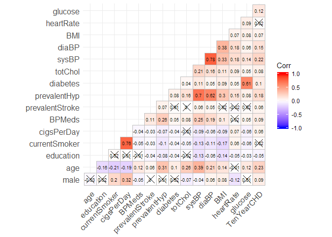
Lets look at some correlations that are higher than 0.70. Correlations below 0.70 can be assumed to not affect our analysis.
- currentSmoker and cigsPerDay are highly correlated (0.76)
- sysBP and diaBP are highly correlated (0.78)
- prevalentHyp and sysBP are highly correlated (0.70)
How does our Variable of Interest affect our dependent variable?
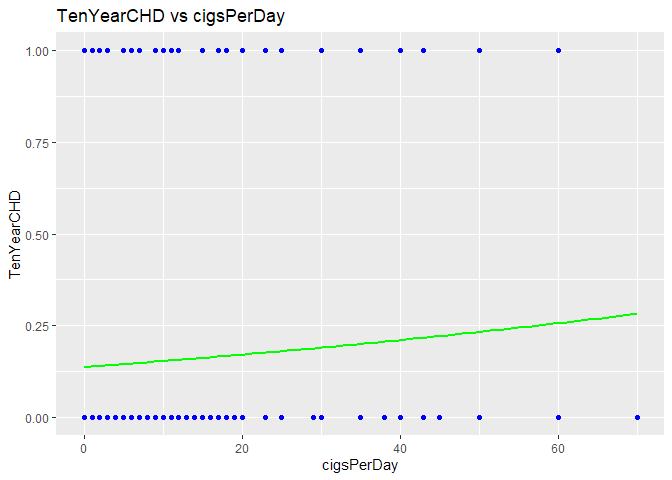
From our expectations, an increase in the number of cigarettes per day should increase the risk of getting coronary heart disease.
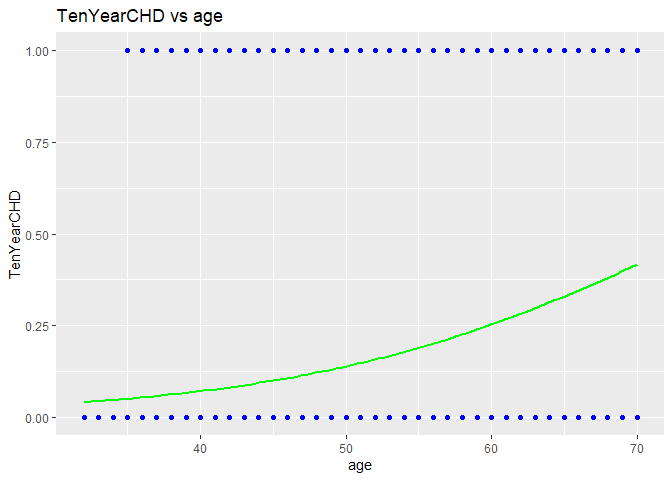
From the plot between Age and dependent variable, it appears as age increases, the risk of getting Coronary Heart Disease increases. Lets see how age relates to cigsPerDay (variable of interest).
Correlation (X, Z): -0.1918467
Now, when given a single argument to anova, it produces a table which tests whether the model terms are significant. So, through the line of code shown above, we are trying to show how ‘age’ relates to our variable of interest (cigsPerDay). From the results we can see that not only age is negatively correlated with cigsPerDay, but also significant with 95% confidence. Thus establishing the relevance that corr (X, Z) < 0.
- As Z(age) affects Y positively, and corr(X,Z) < 0, we suspect presence of downward bias.
- From the model-2 results, we see that adding Age increased estimate of cigsPerDay, suggesting that model1 suffered from downward bias.
- Pseudo R-square increases to 0.07345529.
Interpretation:
- Logit1 -
- cigsPerDay: An increase in cigarettes smoked per day by 1, on average, will increase the chance of CHD by 0.2%.
- Logit2 -
- cigsPerDay: Keeping all other things constant, an increase in cigarettes smoked per day by 1, on average, will increase the chance of CHD by 0.3%.
- age: Keeping all other things constant, an increase in age by 1 year, on average will increase the chance of CHD by 1.0%.
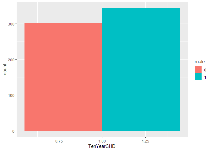
From the plot between Male and dependent variable, it appears that the risk of getting Coronary Heart Disease increases is greater for males than females.
Lets see how male relates to cigsPerDay (variable of interest).
Correlation (X, Z): 0.3156298
Now, when given a single argument to anova, it produces a table which tests whether the model terms are significant. So, we are trying to show how ‘male’ relates to our variable of interest (cigsPerDay). From the results we can see that not only male is positively correlated with cigsPerDay, but also significant with 95% confidence. Thus establishing the relevance that corr (X, Z) > 0.
- As Z(male) affects Y positively, and corr(X,Z) > 0, we suspect presence of upward bias.
- From the model-3 results, we see that adding Male decreased estimate of cigsPerDay, suggesting that model2 suffered from upward bias. Pseudo R-square increases from 0.07345529 to 0.07848801.
Interpretation:
- Logit2 -
- cigsPerDay: Keeping all other things constant, an increase in cigarettes smoked per day by 1, on average, will increase the chance of CHD by 0.3%.
- age: Keeping all other things constant, an increase in age by 1 year, on average will increase the chance of CHD by 1.0%.
- Logit3 -
- cigsPerDay: Keeping all other things constant, an increase in cigarettes smoked per day by 1, on average, will increase the chance of CHD by 0.2%.
- age: Keeping all other things constant, an increase in age by 1 year, on average will increase the chance of CHD by 0.9%.
- male: Keeping all other things constant, on average, Males have higher risk of CHD than Females by 4.6%.
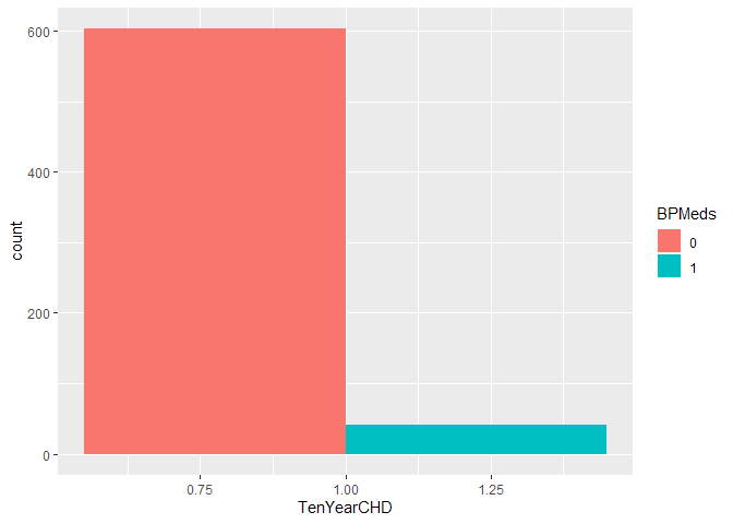
Lets see how BPMeds relates to cigsPerDay (variable of interest).
Correlation (X, Z): -0.04467498
Now, when given a single argument to anova, it produces a table which tests whether the model terms are significant. So, we are trying to show how ‘BPMeds’ relates to our variable of interest (cigsPerDay). From the results we can see that not only BPMeds is negatively correlated with cigsPerDay, but also significant with 95% confidence. Thus establishing the relevance that corr (X, Z) < 0.
- As Z(BPMeds) affects Y positively, and corr(X,Z) < 0, we suspect presence of downward bias.
- From the model-4 results, we see that adding BPMeds increased estimate of cigsPerDay, suggesting that model3 suffered from downward bias.
- Pseudo R-square increases from 0.07848801 to 0.08244846.
Interpretation:
- Logit3 -
- cigsPerDay: Keeping all other things constant, an increase in cigarettes smoked per day by 1, on average, will increase the chance of CHD by 0.2%.
- age: Keeping all other things constant, an increase in age by 1 year, on average will increase the chance of CHD by 0.9%.
- male: Keeping all other things constant, on average, Males have higher risk of CHD than Females by 4.6%.
- Logit4 -
- cigsPerDay: Keeping all other things constant, an increase in cigarettes smoked per day by 1, on average, will increase the chance of CHD by 0.2%.
- age: Keeping all other things constant, an increase in age by 1 year, on average will increase the chance of CHD by 0.9%.
- male: Keeping all other things constant, on average, Males have higher risk of CHD than Females by 4.9%.
- BPMeds: Keeping all other things constant, on average, a person on BP Medication has a higher risk of CHD than a person not on BP Medication by 11.9%.
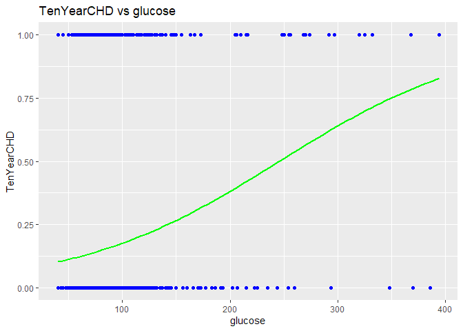
From the plot between glucose and dependent variable, it appears as levels of glucose increase, the risk of getting Coronary Heart Disease increases.
Lets see how glucose relates to cigsPerDay (variable of interest).
Correlation (X, Z): -0.05686326
Now, when given a single argument to anova, it produces a table which tests whether the model terms are significant. So, through the line of code shown above, we are trying to show how ‘glucose’ relates to our variable of interest (cigsPerDay). From the results we can see that not only glucose is negatively correlated with cigsPerDay, but also significant with 95% confidence. Thus establishing the relevance that corr (X, Z) < 0.
- As Z(glucose) affects Y positively, and corr(X,Z) < 0, we suspect presence of downward bias.
- From the model-5 results, we see that adding glucose increased the estimate of cigsPerDay, suggesting that model4 suffered from downward bias.
- Pseudo R-square increases from 0.08244846 to 0.09045346.
Interpretation:
- Logit4 -
- cigsPerDay: Keeping all other things constant, an increase in cigarettes smoked per day by 1, on average, will increase the chance of CHD by 0.2%.
- age: Keeping all other things constant, an increase in age by 1 year, on average will increase the chance of CHD by 0.9%.
- male: Keeping all other things constant, on average, Males have higher risk of CHD than Females by 4.9%.
- BPMeds: Keeping all other things constant, on average, a person on BP Medication has a higher risk of CHD than a person not on BP Medication by 11.9%.
- Logit5 -
- cigsPerDay: Keeping all other things constant, an increase in cigarettes smoked per day by 1, on average, will increase the chance of CHD by 0.2%.
- age: Keeping all other things constant, an increase in age by 1 year, on average will increase the chance of CHD by 0.9%.
- male: Keeping all other things constant, on average, Males have higher risk of CHD than Females by 4.8%.
- BPMeds: Keeping all other things constant, on average, a person on BP Medication has a higher risk of CHD than a person not on BP Medication by 11.2%.
- glucose: Keeping all other things constant, an increase in glucose level by 1 mg/DL, on average, will increase the risk of CHD by 0.1%.
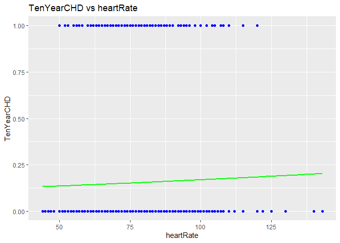
From the plot between heartRate and dependent variable, it appears as heartRate increases, the risk of getting Coronary Heart Disease increases. Lets see how heartRate relates to cigsPerDay (variable of interest).
Correlation (X, Z): 0.07385272
Now, when given a single argument to anova, it produces a table which tests whether the model terms are significant. So, through the line of code shown above, we are trying to show how ‘heartRate’ relates to our variable of interest (cigsPerDay). From the results we can see that not only heartRate is positively correlated with cigsPerDay, but also significant with 95% confidence. Thus establishing the relevance that corr (X, Z) > 0.
- As Z(heartRate) affects Y positively, and corr(X,Z) > 0, we suspect presence of upward bias.
- From the model-6 results, we see that adding heartRate decreased the estimate of cigsPerDay, suggesting that model5 suffered from upward bias.
- Pseudo R-square increases from 0.09045346 to 0.0909557.
Interpretation:
- Logit5 -
- cigsPerDay: Keeping all other things constant, an increase in cigarettes smoked per day by 1, on average, will increase the chance of CHD by 0.2%.
- age: Keeping all other things constant, an increase in age by 1 year, on average will increase the chance of CHD by 0.9%.
- male: Keeping all other things constant, on average, Males have higher risk of CHD than Females by 4.8%.
- BPMeds: Keeping all other things constant, on average, a person on BP Medication has a higher risk of CHD than a person not on BP Medication by 11.2%.
- glucose: Keeping all other things constant, an increase in glucose level by 1 mg/DL, on average, will increase the risk of CHD by 0.1%.
- Logit6 -
- cigsPerDay: Keeping all other things constant, an increase in cigarettes smoked per day by 1, on average, will increase the chance of CHD by 0.2%.
- age: Keeping all other things constant, an increase in age by 1 year, on average will increase the chance of CHD by 0.9%.
- male: Keeping all other things constant, on average, Males have higher risk of CHD than Females by 5.0%.
- BPMeds: Keeping all other things constant, on average, a person on BP Medication has a higher risk of CHD than a person not on BP Medication by 11.1%.
- glucose: Keeping all other things constant, an increase in glucose level by 1 mg/DL, on average, will increase the risk of CHD by 0.1%.
- heartRate: Keeping all other things constant, an increase in heartRate by 1 unit, on average, will increase the risk of CHD by 0.1%.
Correlation (Y, Z): 0.090405
We see that interaction term positively affects Y.
Lets see how heartRate relates to cigsPerDay (variable of interest).
Correlation (X, Z): -0.0519312
Now, when given a single argument to anova, it produces a table which tests whether the model terms are significant. So, we are trying to show how interaction term relates to our variable of interest (cigsPerDay). From the results we can see that the interaction is negatively correlated with cigsPerDay, but is not significant. Thus we can not establish the relevance that corr (X, Z) < 0.
- As Z(interaction term) affects Y positively, and corr(X,Z) < 0 (not significant), we suspect presence of downward bias.
- Adding prevalentStroke*BPMeds did not change the estimate of cigsPerDay, suggesting that model6 did not suffer from bias.
- Pseudo R-square increases from 0.0909557 to 0.09408247.
Interpretation:
- Logit6 -
- cigsPerDay: Keeping all other things constant, an increase in cigarettes smoked per day by 1, on average, will increase the chance of CHD by 0.2%.
- age: Keeping all other things constant, an increase in age by 1 year, on average will increase the chance of CHD by 0.9%.
- male: Keeping all other things constant, on average, Males have higher risk of CHD than Females by 5.0%.
- BPMeds: Keeping all other things constant, on average, a person on BP Medication has a higher risk of CHD than a person not on BP Medication by 11.1%.
- glucose: Keeping all other things constant, an increase in glucose level by 1 mg/DL, on average, will increase the risk of CHD by 0.1%.
- heartRate: Keeping all other things constant, an increase in heartRate by 1 unit, on average, will increase the risk of CHD by 0.1%.
- Logit7 -
- cigsPerDay: Keeping all other things constant, an increase in cigarettes smoked per day by 1, on average, will increase the chance of CHD by 0.2%.
- age: Keeping all other things constant, an increase in age by 1 year, on average will increase the chance of CHD by 0.9%.
- male: Keeping all other things constant, on average, Males have higher risk of CHD than Females by 5.0%.
- BPMeds: Keeping all other things constant, on average, a person on BP Medication has a higher risk of CHD than a person not on BP Medication by 12.1%.
- glucose: Keeping all other things constant, an increase in glucose level by 1 mg/DL, on average, will increase the risk of CHD by 0.1%.
- heartRate: Keeping all other things constant, an increase in heartRate by 1 unit, on average, will increase the risk of CHD by 0.1%.
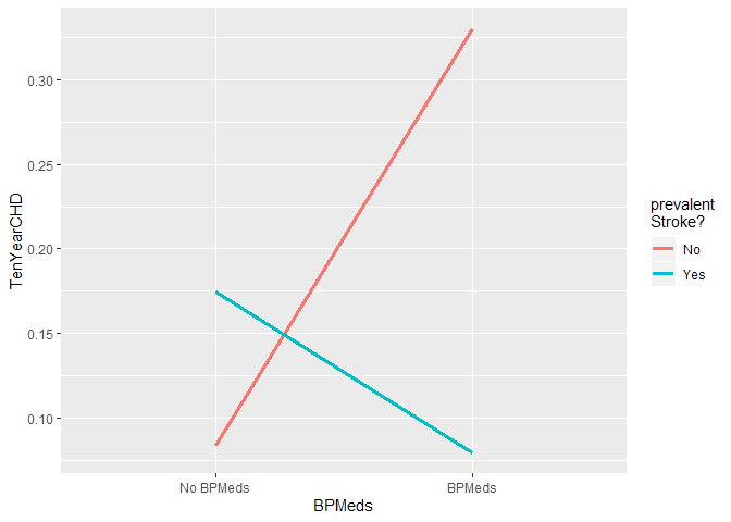
- prevalentStroke: Keeping all other things constant, on average a person with prevalent history of stroke is 30.9% more likely to have CHD.
- I(BPMeds–prevalentStroke): Keeping all other things constant, the impact of prevalentStroke on CHD, on average, decreases by 11.6% for patients that are on BP Medication.
After adding the Interaction term in Model 7 ,the value of β1^ didn’t change . Let’s compare Model 6 and Model 7 using Chi- Square Test to find the better model .
HO:β1=0 and β2=0 and β3=0 and β4=0 and β5=0 and β6=0,
HA:β1 ≠ 0 and/or β2 ≠ 0 and/or β3 ≠ 0 and/or β4 ≠ 0 and/or β5 ≠ 0 and/or β6 ≠ 0 and/or β7 ≠ 0
Pr(>Chi) = 0.003531 **
The probability of seeing a difference is 0.003530654 which is less than 0.05 (which is the alpha level associated with a 95% confidence level).
The small p-value from the Chi-squared test would lead us to conclude that at least one of the regression coefficients in the model is not equal to zero.
Thus, we can reject the null hypothesis that coefficients are zero at any level of significance commonly used in practice.
From our analytical study, we can conclude the consistent evidence supporting a causal role of smoking in causing coronary heart disease. Thus establishing a causal relationship between the two.
---------Logit1 Logit2 Logit3 Logit4 Logit5 Logit6 Logit7
cigsPerDay 0.013 0.026 0.020 0.021 0.022 0.021 0.021
β1^= 0.021 (significant with 95% confidence) Marginal Effect of β1 = 0.002
Looking at our model, we can say: For every extra cigarette smoked, on average, the risk of getting CHD (over the course of next 10 years) will increase by 0.2%, holding other variables constant.
- Threats to Internal Validity :
- Omitted variable Bias : Added control variables till the estimate β1 was consistent.
- Misspecification of the functional form : Dependent variable is binary, so we used Logit.
- Measurement errors : Could be present, not enough information to account for it.
- Missing data and sample selection : Imputed missing values using mean() and median() methods after checking for outliers in the variables of interest.
- Threats to External Validity:
- Differences in populations : Estimated results for 10YearCHD using data from Framingham, MA, USA might not hold true for some other country like India with individuals having high risk of heart related diseases. Eg: Diets are completely different along with their medical conditions.
- Differences in settings : Diagnostic and treatment procedures may vary.