HarlinLee / BlobOT

A Blob Method for Mean Field Control with Terminal Constraints

BlobOT

Python code for the paper A Blob Method for Mean Field Control with Terminal Constraints by Katy Craig, Karthik Elamvazhuthi, and Harlin Lee.

What's inside?

BlobOT.py contains the most important class and function definitions for the optimization problem.

• Model is (more or less) a dummy class so that we can leverage the autograd functionality of Pytorch.
• KE calculates the kinetic energy using velocity of the trajectories.
• KE_acc uses the acceleration of trajectories.
• Use NLE to calcualte the non-local energy term (without $m_1^2$, so this may be negative) when the target distribution is an empirical distribution. We assume equal weights per particle, but that should be easily modifiable if you need to.
• NLE_acc is for the acceleration control example. It needs special treatment to deal with position and velocity becoming a $d+1$-dimensional vector together.
• NLE_gauss is the contiuum Gaussian distribution version of NLE.
• NLE_cons calculates $m_1^2$, the term that's always positive and doesn't affect the optimization problem. For large $N$, it would make sense to modify the code such that this is calculated only once.
• NLE_pos and NLE_acc_pos come in handy if you want to calculate the non-negative version of the NLE, e.g. for a log-log plot.
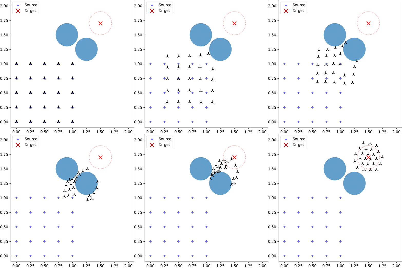
• obstacle calculates how much cost is incurred by the current trajectory with respect to one circular obstacle.

The following notebooks can be run after cloning this repo and installing Pytorch. Every figure, npz and pkl file created by this repo should be in the output folder. If any are missing (such as small_eps_{date}.npz), it's because the file was too large for github.

• loss_contour.ipynb
• diff_eps.ipynb: This may produce a different output due to randomness, but it should be qualitatively the same.
• small_eps.ipynb: Run this file after diff_eps.ipynb because this uses the same source and target distributions as the previous experiment.
• delta_scaling.ipynb
• POT_comparison.ipynb: This may produce a different output due to randomness.
• continuum_gaussian.ipynb: The empirical distribution version may produce a different output due to randomness.
• obstacles.ipynb
• acceleration.ipynb: The shuffled velocity experiment may produce a different output due to randomness.

Helpful tips:

• blobLoss and training_loop are written so that they are easily adaptable to other examples.
• z and w are the source and target distributions, respectively.
• y denotes $x(1)$, i.e. particle positions at $t=1$.
• Even though we use the method torch.optim.SGD, it's actually GD and not SGD.
• X0 and X inside the model is of length $L = 1/\Delta t$ in the time dimension and does not include $z = x(0)$. They're of the shape $N \times d \times L$, or particles x dimension x time steps.
• The use of npz vs. pkl is pretty random.