pyGAM
Generalized Additive Models in Python.
Installation
pip install pygam
scikit-sparse
To speed up optimization on large models with constraints, it helps to have scikit-sparse installed because it contains a slightly faster, sparse version of Cholesky factorization. The import from scikit-sparse references nose, so you'll need that too.
The easiest way is to use Conda:
conda install scikit-sparse nose
About
Generalized Additive Models (GAMs) are smooth semi-parametric models of the form:
where X.T = [X_1, X_2, ..., X_p] are independent variables, y is the dependent variable, and g() is the link function that relates our predictor variables to the expected value of the dependent variable.
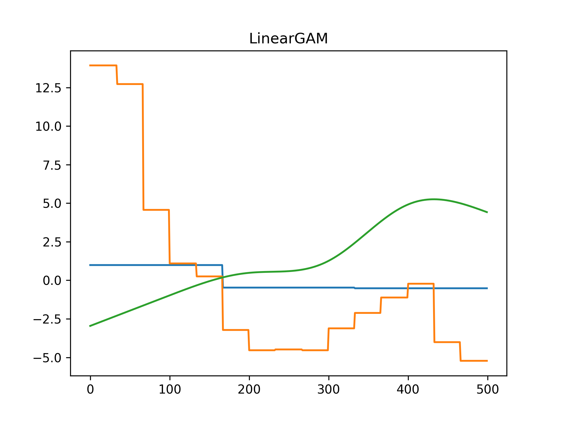
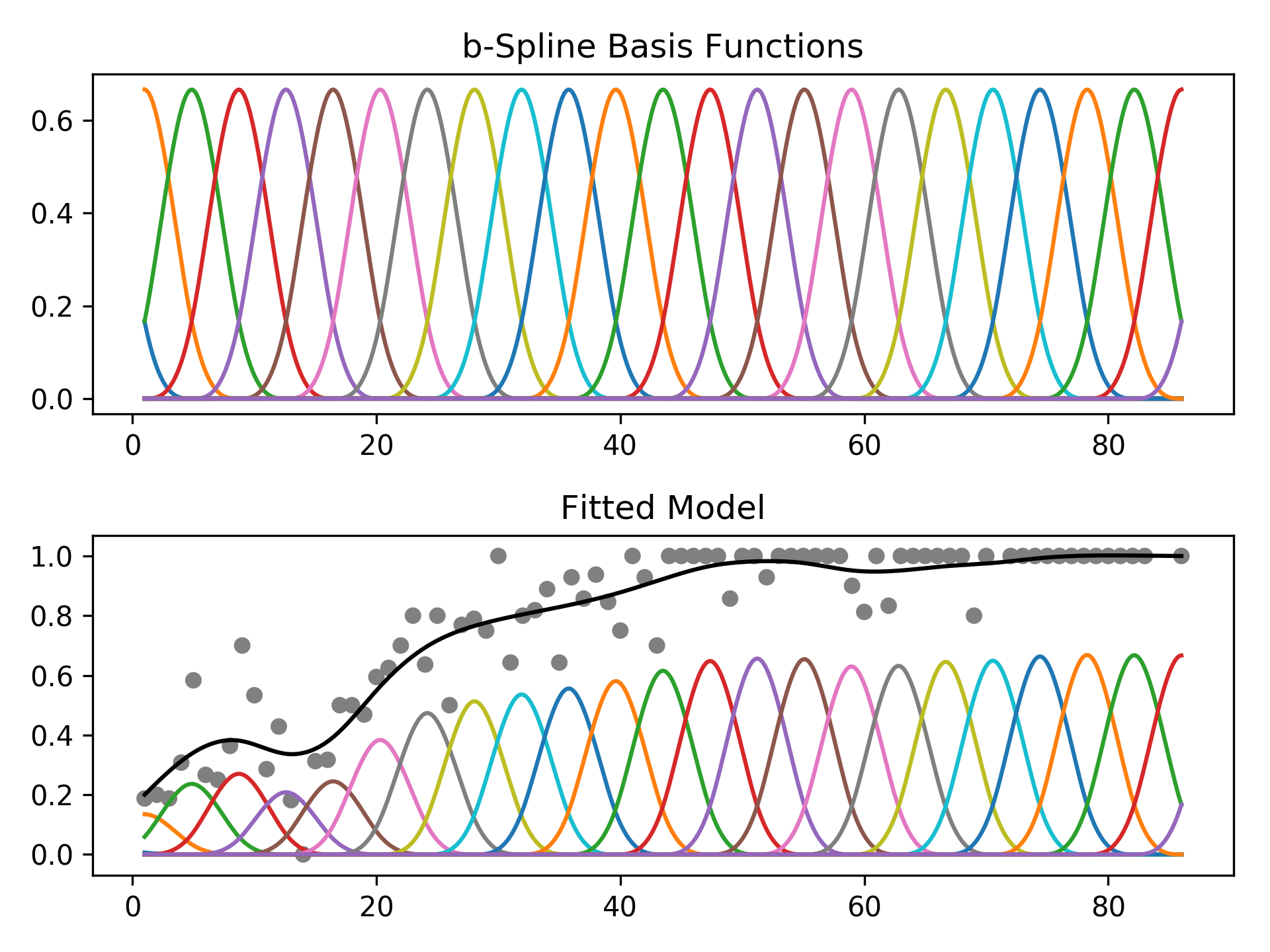
The feature functions f_i() are built using penalized B splines, which allow us to automatically model non-linear relationships without having to manually try out many different transformations on each variable.
GAMs extend generalized linear models by allowing non-linear functions of features while maintaining additivity. Since the model is additive, it is easy to examine the effect of each X_i on Y individually while holding all other predictors constant.
The result is a very flexible model, where it is easy to incorporate prior knowledge and control overfitting.
Regression
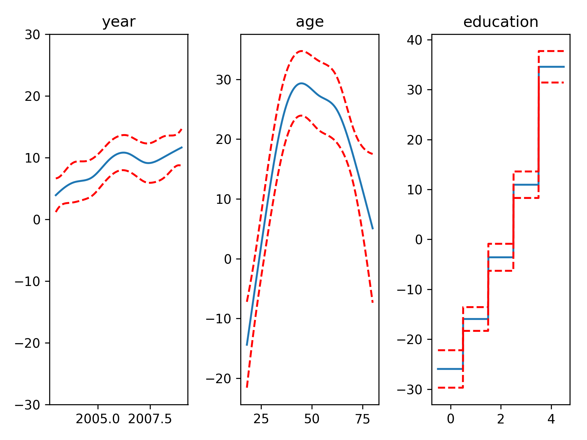
For regression problems, we can use a linear GAM which models:
# wage dataset
from pygam import LinearGAM
from pygam.utils import generate_X_grid

gam = LinearGAM(n_splines=10).gridsearch(X, y)
XX = generate_X_grid(gam)

fig, axs = plt.subplots(1, 3)
titles = ['year', 'age', 'education']

for i, ax in enumerate(axs):
    pdep, confi = gam.partial_dependence(XX, feature=i+1, width=.95)

    ax.plot(XX[:, i], pdep)
    ax.plot(XX[:, i], confi, c='r', ls='--')
    ax.set_title(titles[i])
Even though we allowed n_splines=10 per numerical feature, our smoothing penalty reduces us to just 14 effective degrees of freedom:
gam.summary()

Model Statistics
------------------
edof        14.087
AIC      29889.895
AICc     29890.058
GCV       1247.059
scale     1236.523

Pseudo-R^2
----------------------------
explained_deviance     0.293
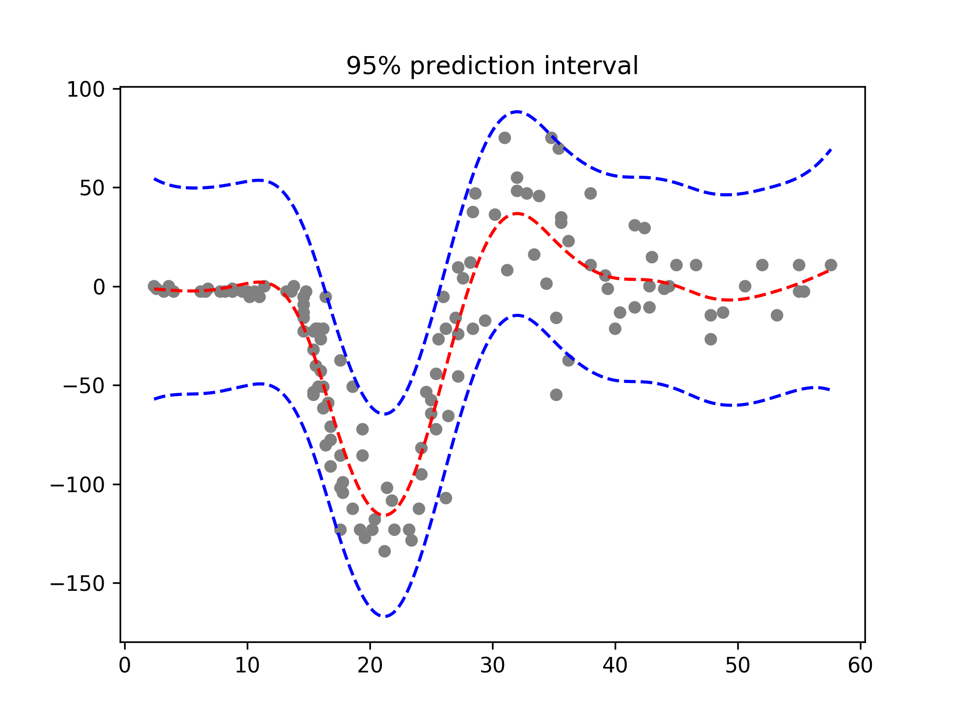
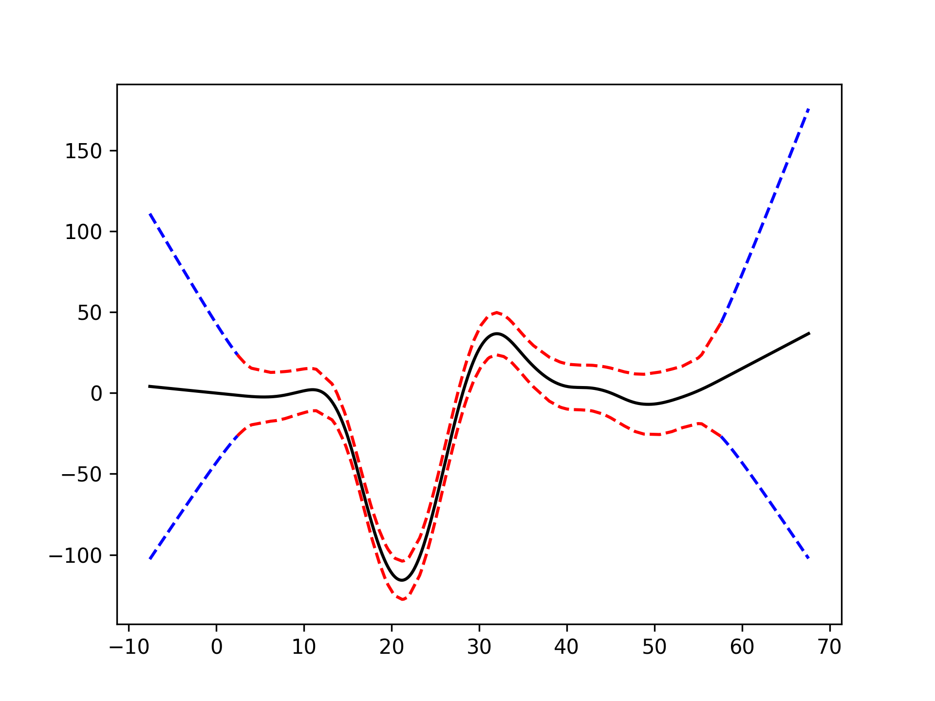
With LinearGAMs, we can also check the prediction intervals:
# mcycle dataset
from pygam import LinearGAM
from pygam.utils import generate_X_grid

gam = LinearGAM().gridsearch(X, y)
XX = generate_X_grid(gam)

plt.plot(XX, gam.predict(XX), 'r--')
plt.plot(XX, gam.prediction_intervals(XX, width=.95), color='b', ls='--')

plt.scatter(X, y, facecolor='gray', edgecolors='none')
plt.title('95% prediction interval')
Classification
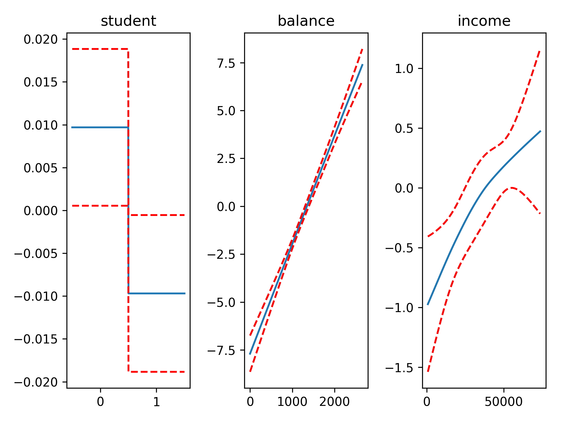
For binary classification problems, we can use a logistic GAM which models:
# credit default dataset
from pygam import LogisticGAM
from pygam.utils import generate_X_grid

gam = LogisticGAM().gridsearch(X, y)
XX = generate_X_grid(gam)

fig, axs = plt.subplots(1, 3)
titles = ['student', 'balance', 'income']

for i, ax in enumerate(axs):
    pdep, confi = gam.partial_dependence(XX, feature=i+1, width=.95)

    ax.plot(XX[:, i], pdep)
    ax.plot(XX[:, i], confi, c='r', ls='--')
    ax.set_title(titles[i])
We can then check the accuracy:
gam.accuracy(X, y)

0.97389999999999999
Since the scale of the Bernoulli distribution is known, our gridsearch minimizes the Un-Biased Risk Estimator (UBRE) objective:
gam.summary()

Model Statistics
----------------
edof       4.364
AIC     1586.153
AICc     1586.16
UBRE       2.159
scale        1.0

Pseudo-R^2
---------------------------
explained_deviance     0.46
Poisson and Histogram Smoothing
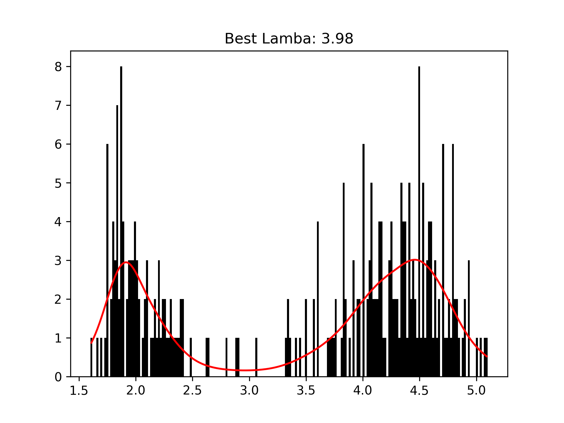
We can intuitively perform histogram smoothing by modeling the counts in each bin as being distributed Poisson via PoissonGAM.
# old faithful dataset
from pygam import PoissonGAM

gam = PoissonGAM().gridsearch(X, y)

plt.plot(X, gam.predict(X), color='r')
plt.title('Lam: {0:.2f}'.format(gam.lam))
Custom Models
It's also easy to build custom models, by using the base GAM class and specifying the distribution and the link function.
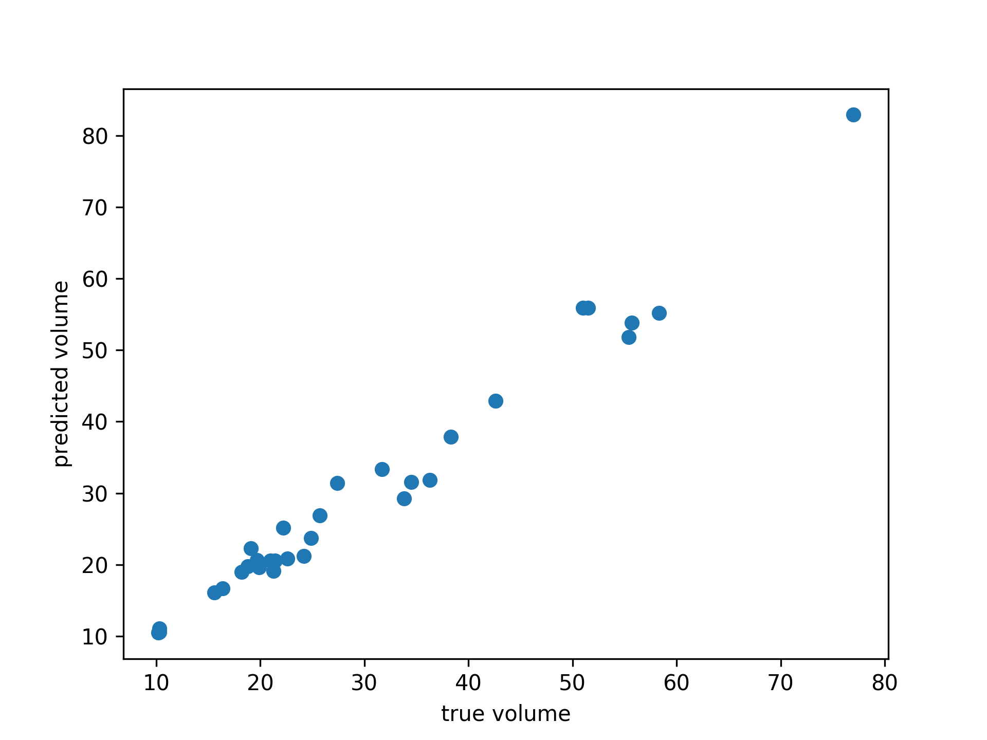
# cherry tree dataset
from pygam import GAM

gam = GAM(distribution='gamma', link='log', n_splines=4)
gam.gridsearch(X, y)

plt.scatter(y, gam.predict(X))
plt.xlabel('true volume')
plt.ylabel('predicted volume')
We can check the quality of the fit:
gam.summary()

Model Statistics
----------------
edof       4.154
AIC      144.183
AICc     146.737
GCV        0.009
scale      0.007

Pseudo-R^2
----------------------------
explained_deviance     0.977
Penalties / Constraints
With GAMs we can encode prior knowledge and control overfitting by using penalties and constraints.
Available penalties:
- second derivative smoothing (default on numerical features)
- L2 smoothing (default on categorical features)
Availabe constraints:
- monotonic increasing/decreasing smoothing
- convex/concave smoothing
- periodic smoothing [soon...]
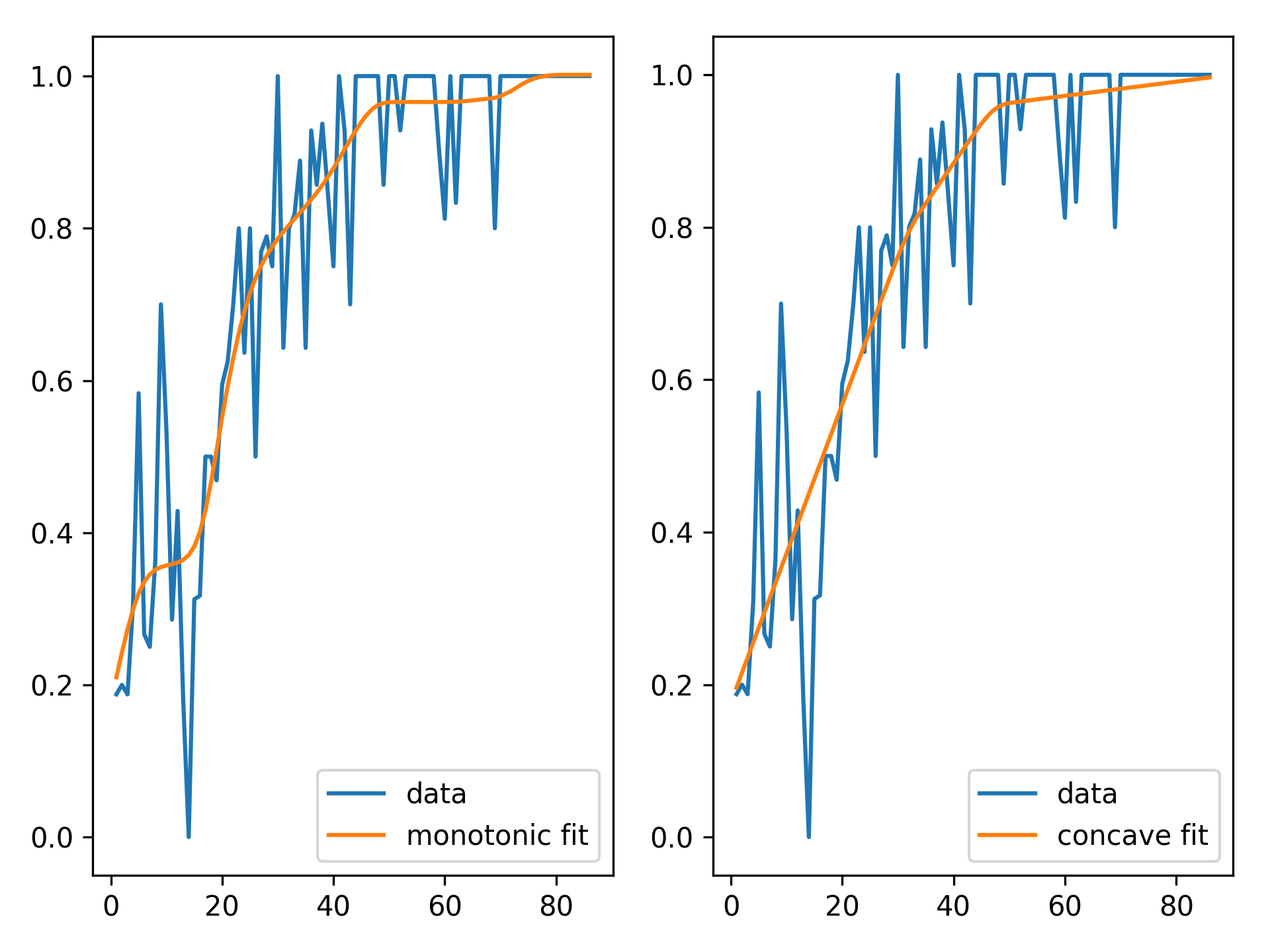
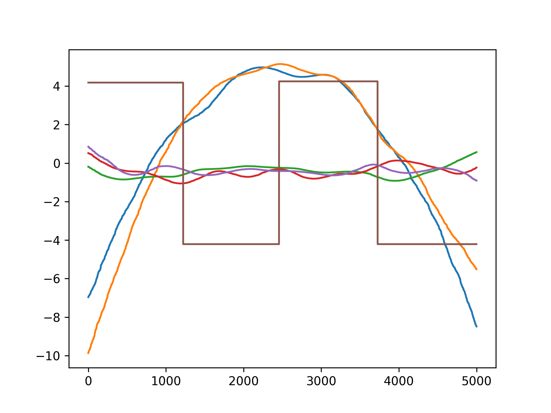
We can inject our intuition into our model by using monotonic and concave constraints:
# hepatitis dataset
from pygam import LinearGAM

gam1 = LinearGAM(constraints='monotonic_inc').fit(X, y)
gam2 = LinearGAM(constraints='concave').fit(X, y)

fig, ax = plt.subplots(1, 2)
ax[0].plot(X, y, label='data')
ax[0].plot(X, gam1.predict(X), label='monotonic fit')
ax[0].legend()

ax[1].plot(X, y, label='data')
ax[1].plot(X, gam2.predict(X), label='concave fit')
ax[1].legend()
API
pyGAM is intuitive, modular, and adheres to a familiar API:
from pygam import LogisticGAM

gam = LogisticGAM()
gam.fit(X, y)
Since GAMs are additive, it is also super easy to visualize each individual feature function, f_i(X_i). These feature functions describe the effect of each X_i on y individually while marginalizing out all other predictors:
pdeps = gam.partial_dependence(X)
plt.plot(pdeps)
Current Features
Models
pyGAM comes with many models out-of-the-box:
- GAM (base class for constructing custom models)
- LinearGAM
- LogisticGAM
- GammaGAM
- PoissonGAM
- InvGaussGAM
You can mix and match distributions with link functions to create custom models!
gam = GAM(distribution='gamma', link='inverse')Distributions
- Normal
- Binomial
- Gamma
- Poisson
- Inverse Gaussian
Link Functions
Link functions take the distribution mean to the linear prediction. These are the canonical link functions for the above distributions:
- Identity
- Logit
- Inverse
- Log
- Inverse-squared
Callbacks
Callbacks are performed during each optimization iteration. It's also easy to write your own.
- deviance - model deviance
- diffs - differences of coefficient norm
- accuracy - model accuracy for LogisticGAM
- coef - coefficient logging
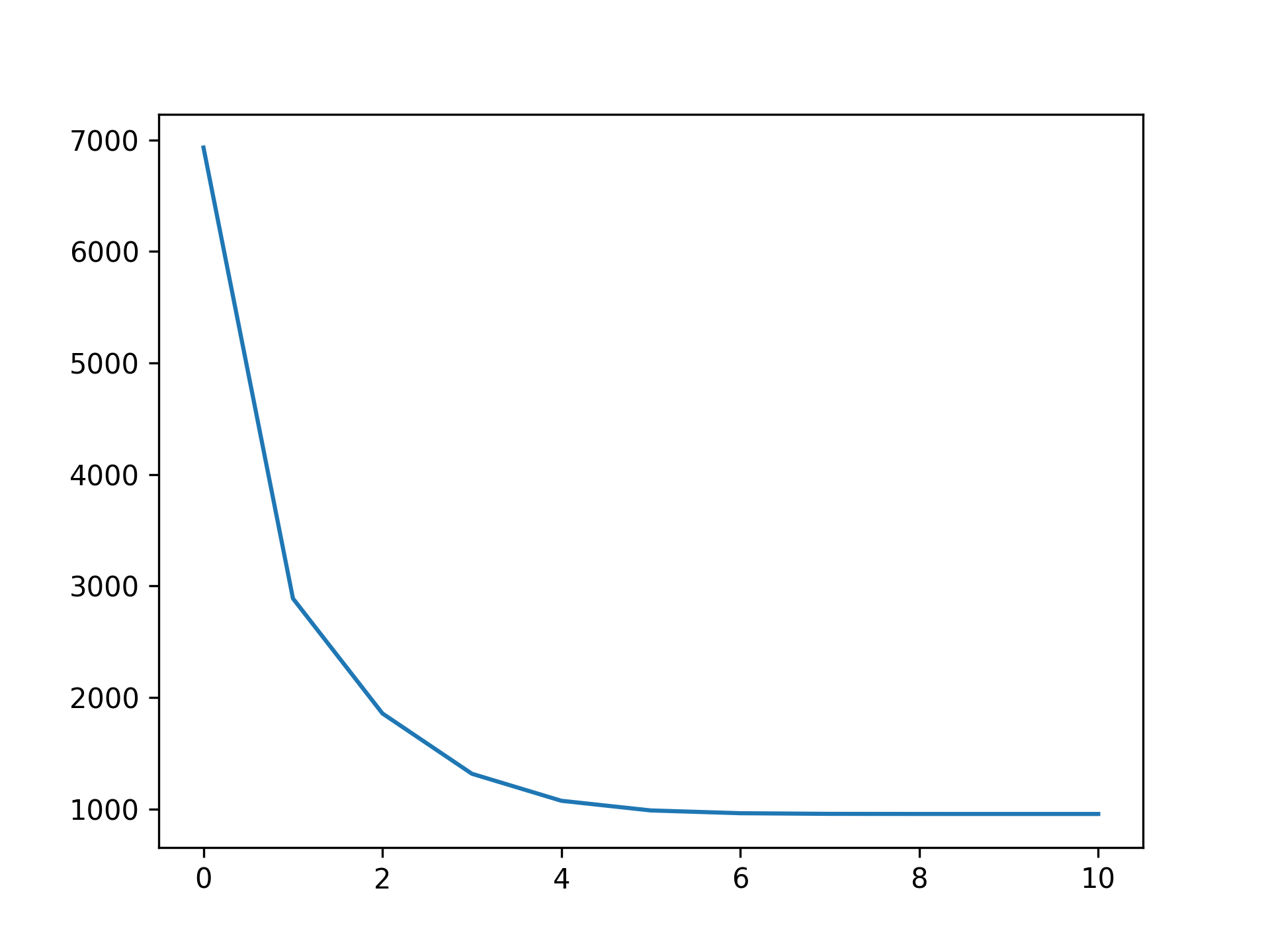
You can check a callback by inspecting:
plt.plot(gam.logs_['deviance'])Linear Extrapolation
References
-
Simon N. Wood, 2006
Generalized Additive Models: an introduction with R -
Hastie, Tibshirani, Friedman
The Elements of Statistical Learning
http://statweb.stanford.edu/~tibs/ElemStatLearn/printings/ESLII_print10.pdf -
James, Witten, Hastie and Tibshirani
An Introduction to Statistical Learning
http://www-bcf.usc.edu/~gareth/ISL/ISLR%20Sixth%20Printing.pdf -
Paul Eilers & Brian Marx, 1996 Flexible Smoothing with B-splines and Penalties http://www.stat.washington.edu/courses/stat527/s13/readings/EilersMarx_StatSci_1996.pdf
-
Kim Larsen, 2015
GAM: The Predictive Modeling Silver Bullet
http://multithreaded.stitchfix.com/assets/files/gam.pdf -
Deva Ramanan, 2008
UCI Machine Learning: Notes on IRLS
http://www.ics.uci.edu/~dramanan/teaching/ics273a_winter08/homework/irls_notes.pdf -
Paul Eilers & Brian Marx, 2015
International Biometric Society: A Crash Course on P-splines
http://www.ibschannel2015.nl/project/userfiles/Crash_course_handout.pdf -
Keiding, Niels, 1991
Age-specific incidence and prevalence: a statistical perspective


