Anonymization of the 1994 US Data Census dataset
The present report, written in the context of PET (Privacy Enhancing Technologies) curricular unit at FCUP (Faculdade de Ciências da Universidade do Porto), aims at describing the process of anonymizing a dense dataset, going from the initial steps of identifying and classifying the dataset attributes, analyzing its re-identification risk, to the chose and appliance of privacy models, performing a comparison between privacy and utility values. The report structure is as follows: first an introduction of the dataset will be done, in order for the reader to be aware of the background information that is inherited in the anonymization process, as well as the established requirements and goals for the anonymization; secondly, configurations defined for the dataset before anonymization will be presented, covering all initial transformations performed to clean the dataset, approaches taken to classify its attributes and the anonymization operations used to transform data. Finally, the last chapter presents an analysis of the obtained results after anonymization, measures taken to refine the results and some final conclusions, as well as future work, for improving the dataset anonymization.
Introduction
The dataset in study represents a small subset of an even bigger dataset: the US Data Census [1]. Census is a form of activity that aims to inquire the citizens of a country, in order to get insights on the quality of life these are having, as well as their pain-points [2]. This way, the government of the inquired country can get feedback from their citizens and in return improve their lives by investing in the country infrastructure [2]. In the case of the US Census, these are conducted every 10 years [3].
Given the background knowledge of what the census are, the team behind this report chose the 1994 US Data Census dataset for three specific reasons: first, it encompasses a large range of data entries (32561) and attributes (14), some of which reduce the number of results in a specific person identification query (e.g., sex, age and race) (1); secondly, with the available attributes, the initial goal of the dataset may be leveraged to specific social-economic concerns such as discrimination, by ranking individuals salary by their race and sex (2); and last but not least, it is classified as the second most popular dataset in the UCI Machine Learning Repository [4], [5] (a well-known source of public datasets, used to train machine learning algorithms and models), as the time of writing this report, which gives us the feeling that the data and concerns in context are of interest by the general public (3).
The dataset has clear goal in mind: allow data analysts to predict if the yearly salary in the US exceeds $50,000, given a fraction of attribute values (hours per week) from the census. This raises a question for the anonymization process: at which level of detail can the original dataset suffer, so that the forecast is not impacted? Not only there is the need to worry about targeting specific individuals based on the attributes of the dataset, but there is also a need to maintain the quality of the dataset so that the predictions are not different before and after the anonymization of the dataset.
Attributes Description
As outlined previously, the dataset is populated by 32561 data entries (i.e., rows), mapped by a set of 14 attributes (i.e., columns). Before attempting to classify the attributes, it is necessary to understand what each of these represent in the dataset. There are several attributes that relate to the individual biological and identity status (age, sex, race, native country, relationship, marital status), social status and education (work class, occupation, weekly work hours, education), as well as the individual net worth (capital gain, capital loss). Although none of these attributes directly identify a specific individual, through the use of additional datasets, it is possible to correlate data, allowing for an indirect identification.
In addition to these attributes, there are other attributes that correspond to the dataset metadata. The first is fnlwgt, which represents an estimate number of individuals which the census believes a specific data entry represents in all census data (i.e., if there are 10,000 individuals in the census with age 35 and race white, then most likely this number would be approximately 10,000) [6], [7]. One thing to note about this variable, is that the community that tackles this dataset for data science purposes, seem to be very confused when interpreting it [7]. Taking this misunderstand in consideration and knowing that it only represents an estimation rather than an exact match, the team behind the report will consider this specific attribute as insensitive.
The second metadata attribute, education-num, represents the school degree (enumeration attribute) in an index table. Since this attribute is redundant, this column will be truncated before anonymization.
In Appendix A it can be found a more detailed overview of these attributes.
Anonymization Process Requirements
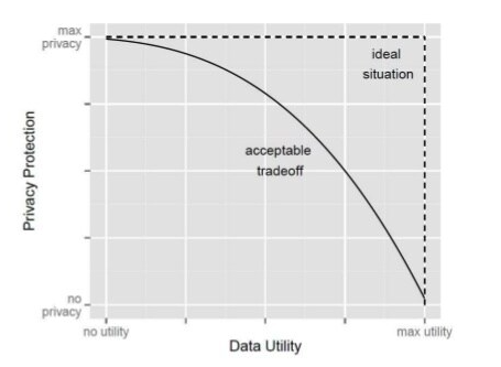
It is known that the goal for the anonymization process is to maintain the quality of the dataset in the sense that it should still be possible to predict if the average yearly salary exceeds $50,000, while making sure that it is not possible to disclose any individual by performing a linkage attack. However, this brings an extra concern for the anonymization process: the trade-off between utility and privacy. The more the dataset privacy is increased, the less utility it will have, due to information loss, as seen below in Figure 1.
To make sure that the utility level of the prediction is not being drastically decreased, there is the need to establish requirements for both utility and privacy levels. For the utility level, it will be used the ML101 kNN Kaggle notebook [9], which uses the k-Nearest-Neighbors algorithm [10] to support the prediction in context. Using the original dataset, the prediction algorithm has an accuracy score of 0.82. With this value in mind, the authors of the report set the following requirement: the utility level after anonymization should not lower more than 10% (i.e., accuracy score should not be lower than 0.738). Additionally, it will be necessary that the utility score of the anonymized dataset should be higher than 70% and the privacy score for re-identification lower than 20%.
ARX and its role on the Anonymization Process
To conduct the anonymization process ARX [11] software will be used. It is an open-source data anonymization tool that has already been used in different industry contexts [12], supporting the whole pipeline for data anonymization: dataset import, attributes classification, re-identification risk analysis, anonymization, coding and privacy models definition and privacy vs utility analysis.
Dataset Anonymization Configuration
Having introduced the dataset background as well as its requirements, a deeper configuration for the anonymization process can be done. This chapter will first start by describing the sanitization procedures applied to the original data. Secondly, a brief classification of the dataset attributes will be made. Subsequentially, the coding models that support attributes transformations will also be described. To conclude, re-identification risks before anonymization will be presented, relating how the analysis of these can help the definition of the privacy parameters.
Data Sanitization
Before importing the dataset to ARX, there is a need to do some sanitization so that it is not polluted during analysis. The original data source of the dataset provides it in a CSV (Comma Separated Value) format [13], which is a supported format in ARX, so no issues on this topic. However, it does not include the attributes names in the first line of the CSV, which is a common practice so that CSV interpreters can then present these in a descriptive way. For this, an extra-line on top of the CSV file was added containing the attribute names.
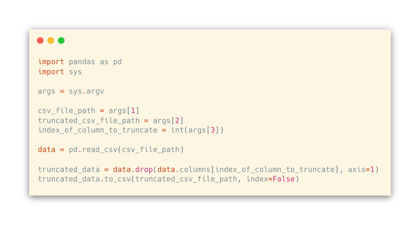
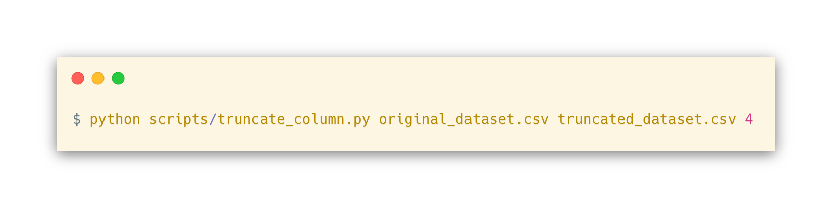
Previously it was described that the attribute education-num was redundant and the column that represents its values needed to be truncated. This could be done in a manual or automated manner. For manual truncation, a platform that allows CSV files manipulation such as Microsoft Excel [14] could be used, requiring the anonymizer to first open the program, import the CSV file, select the column to truncate and then save it. In an automated way, one just needs to write a rather simple program that opens the CSV file, maps it to a list or matrix data structure, indicates which column to remove, and write the new contents back to the file again. With the intention of supporting future anonymizations for both the reader and other entities, the authors of the report decided to stick with the automated manner and create a script using the Python [15] programming language that uses the pandas [16] Python library to help on the CSV manipulation. The script as well its usage on the dataset to remove the education-num column are described below, in Code Snippet 1 and Code Snippet 2.
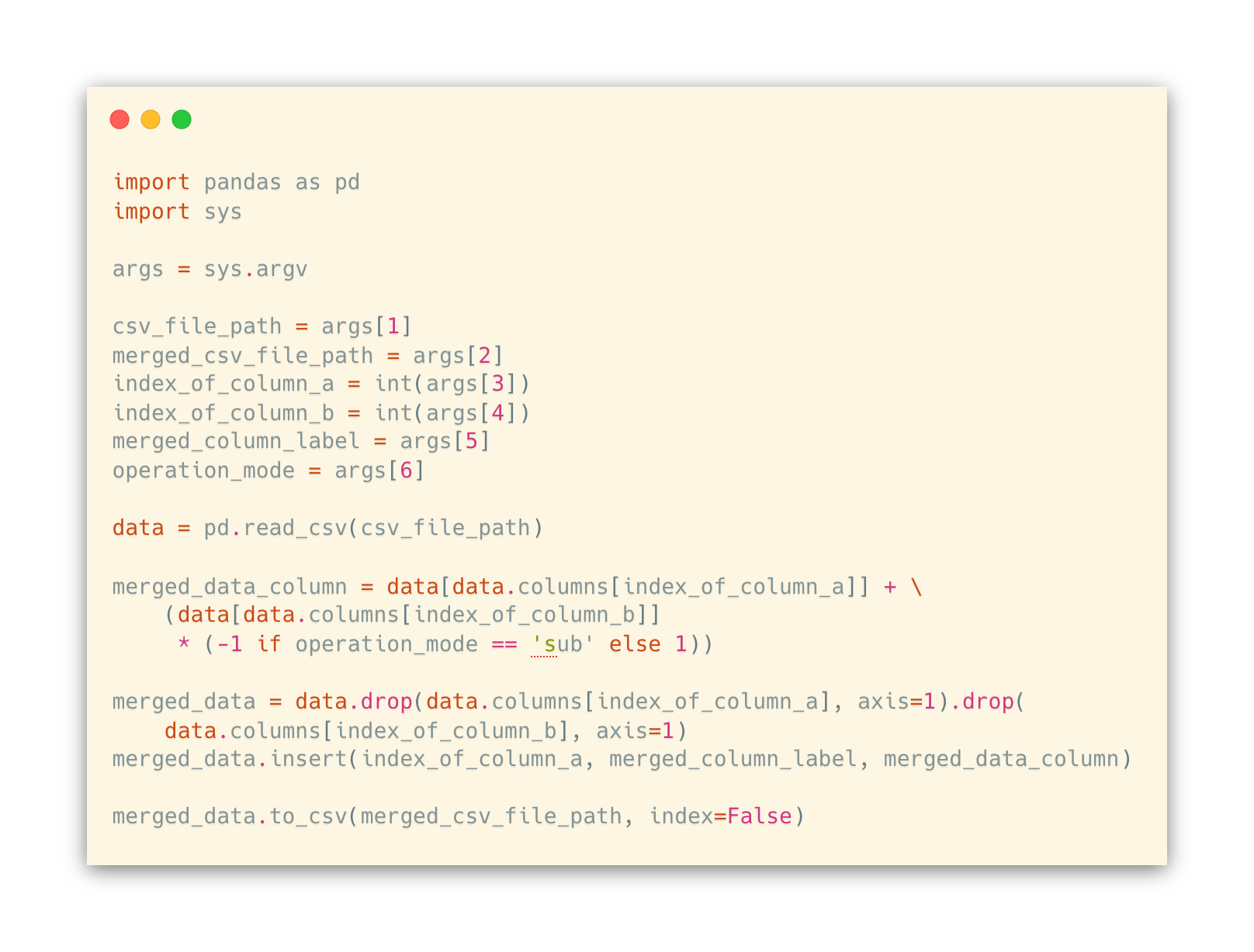
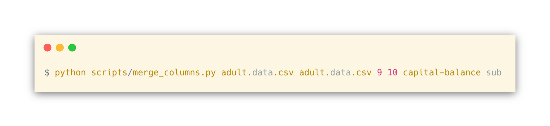
Upon further analysis of the attributes meaning and domains, it was concluded that the attributes capital-gain and capital-loss share the same concept (individual capital balance). In order to reduce the number of columns being anonymized, these two attributes columns were merged in one, which represents the balance of the capital. For this, another Python script that recurs to pandas was created, which requires the indexes of the columns being merged and permits to add or subtract the values being merged (either C = A + B or C = A – B). Again, the source-code and usage of the script can be found below, in Code Snippet 3 and Code Snippet 4 respectively. It is to note that the script only supports numeric columns merge and for this particular scenario, the subtraction (sub) option had to be used, as the capital-loss attribute values are described as positive integers, but in the capital balance domain, it should be interpreted as negative values.
Having sanitized the dataset, it is possible to start classifying its attributes, which will be presented in the next section.
Attributes Classification with support of Risk Analysis
Dataset attributes can be classified in four different types: Identifying, Sensitive, Quasi-Identifying (QID) and Insensitive. Identifying attributes are those who directly reveal an entity in the dataset (e.g., individual name) and so are not available in the final anonymized dataset [11]. For the dataset in context, no direct identifiers were found.
Sensitive attributes represent the data which the data publishers want to directly expose, without suffering any transformation, as these are directly connected to the dataset goal [17]. As previously described, the base goal of the anonymized dataset is to allow the average salary prediction based on the individual hours per week. From this, it is possible to conclude that both the salary (income) and hours per week attributes are sensitive, since these are directly connected to the dataset.
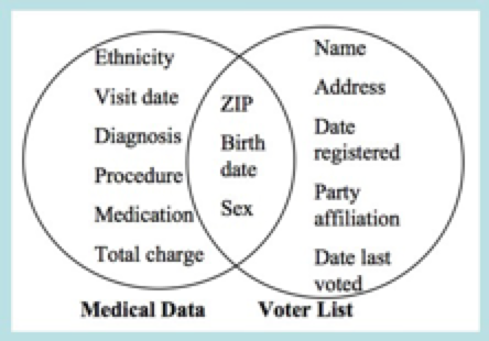
QID attributes when combined with other QID attributes, can be used to identify entities in the dataset, (i.e., indirect identifiers) as these allow for data correlation in re-identification attacks [17]. These can be seen as the intersection of two distinct dataset attributes, as seen in Figure 2.
There are several approaches one can use to identify these attributes. One approach is to pinpoint attributes that are common in different datasets, as these share the same domain concepts which the dataset goal aims to achieve. An example of this is the individual age and sex, since it is something that individuals always have. However, one cannot simply rely on this metric as it can lead to false positives: we, as humans, may think that a specific attribute is a QID since it does not directly identify the individual and it can be present in another dataset, therefore it could be used to correlate the datasets. Anyhow, this is pure speculation and may be heavily influenced by our opinions and as such, the attribute classification is biased.
To prevent this kind of issues, another approach can be followed which relies on statistical analysis of the attribute. For this, two values are calculated: distinction and separation. Distinction tells how unique the values distribution is (e.g., individual names tend to have a higher distinction value, since it is not likely for a group of people to have the same name), while separation tells how unique a pair of attribute values is in comparison to all values present in the distribution (e.g., individual gender tends to have a lower separation value, as the distribution is often short (Male, Female, Other)). The higher these values are, the more confidence one has to say that the attribute is a QID. The following formulas describe how these values are calculated.
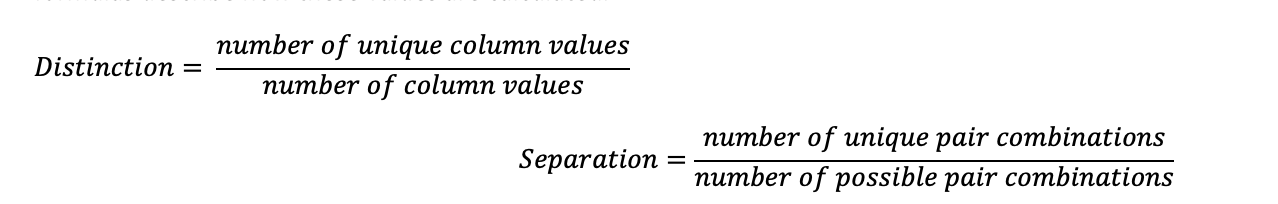
To enhance the QID attributes elicitation and classification, a method that applies both described procedures was defined and used. The method starts by defining the attributes which the anonymizers believe are common in different datasets with equal domains (i.e., base QIDs). Then, add a possible QID attribute for comparison with the base QIDs. Since the anonymizers believe these attributes are QIDs, then it is possible to compare the target attribute values, for both distinction and separation and analyze if these values increase significantly or not. To increase the confidence value, more target attributes should be added in comparison, to check if the distinction and separation values increased significantly. Once an attribute was found to be a potential QID, it is stored in a ranking list that is used to compare with new target attributes, so that a probabilistic metric can take place (e.g., attribute X was admitted as a QID previously with a Y distinct and separation value. When comparing with a new target attribute Z, and it has a distinct and separation value greater than Y, then it is possible to admit that the attribute Z is more probable to be a QID than attribute X).
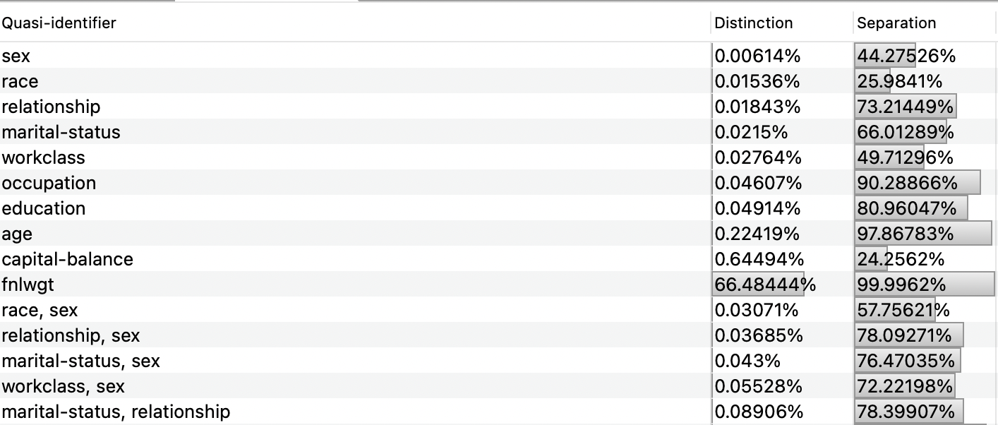
Taking in consideration the defined method for QID attribute classification, the team decided to select attributes age and sex as the base QIDs, as these are attributes that all individuals have. Then, the team started to pick random initial attributes to select one for the ranking list. The education attribute seemed to prove that it is a potential QID, since the difference between its distinct and separation values in combination with the base QIDs was significantly high. Furthermore, occupation and workclass attributes were also compared and it was noticed that both education and occupation attributes have significantly higher values than workclass. Since workclass had the lowest values, it was decided to compare it to the marital-status attribute, which the former showed to have higher distinct values than the latter. This means that marital-status is now the attribute that is ranked as less probable to be a QID.
Race was also an attribute that was considered as a potential QID. Given this, the team compared the attributes age, sex and race and it was noticed that there was a huge discrepancy in the comparison of pairs (age, sex), (age, race) and (sex, race). This led the team to disapprove the idea that race as a QID. Attribute native-country was also a surprise since this value had a separation value of 19% and the values domain was quite big (41 possibilities), meaning that it was less likely to have lower separation values than the sex attribute, which has a binary domain. For that reason, this attribute was also discarded to be a potential QID.
Capital-balance attribute proved to have a distinct value greater than age (the highest so far) but had very low separation values (24%). Upon further analysis of the dataset, it was possible to conclude that this is expected, since there a lot zero (0) values. Given such data discrepancy, it was not possible to properly conclude if the attribute is a QID or not.
Last-but-least, the relationship attribute was compared with the less probable QID in the ranking list, marital-status. Surprisingly, relationship had lower values. Upon further analysis of the attribute distribution, Husband had the highest relevance (~40%), while Wife had the last but one relevance (~4%), meaning that it is not possible this attribute with the sex attribute, considering that Husband corresponds to Male and Wife to Female. For this reason, relationship was discarded as a potential QID, while marital-status was considered.
Insensitive attributes, also known as other attributes, are those attributes that were not classified as either Identifying, QID or Sensitive. As such, these do not represent a big risk for the dataset privacy, not needing to be modified. In Chapter 1, it was described that the attribute fnlwgt represents an estimative of the number of individuals which the dataset entry may represent in all census data. Knowing that it is an estimative, an attacker cannot precisely correlate an entry in the dataset as it is not an exact value. Additionally, the lowest and highest values this attribute can take is 12285 and 1484705 respectively, which supports even more the idea of correlation imprecision, as to guess an individual, it would require to filter a lot of entries.
Furthermore, the remaining attributes that were not classified as QID (race, capital-balance, native-country, relationship) are then considered insensitive.
Anonymization Operations Definition and Coding Model Configuration
As described before, QIDs are transformed during the anonymization process. To allow this transformation, anonymization operations need to be defined and properly configured to meet these attributes specifications. These operations vary in four different categories:
- Generalization, which attempts to transform data in a way that is not so specific, through the creation of hierarchy trees that generalize the domain in levels [19]. Deeper levels are more specific, whereas higher levels are more general;
- Suppression, whereas the name says, specific data is removed from the dataset. This model is particularly useful when combining with generalization, as the latter might lead to too much information loss (i.e., vague data) [19];
- Anatomization, which in contrast to generalization and suppression, does not modify data but instead de-associates QIDs and sensitive attributes, creating association tables which are referenced in the dataset by a numeric identifier [19];
- Random perturbation, where the transforming data is replaced with synthetic statistical values such as noise [19].
For the classified QIDs, the authors of the report decided to focus on generalization and suppression, by creating interval, masking and order-based hierarchies, and balancing the generalization-suppression values. Interval-based hierarchies are specifically useful for numeric distributions as these can be divided given a ratio scale [11]. For this reason, an interval hierarchy for the attribute age was defined, which is the only QID with a numerical scale.
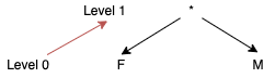
For attribute sex, a masking-based hierarchy was defined, as these are especially useful for attributes which domain cannot be generalized in levels. Instead, information is hidden by applying a mask (typically character ‘*’) to the string characters.
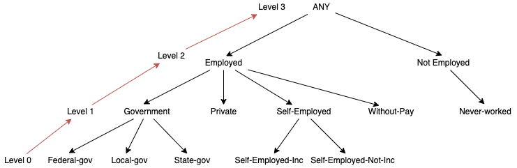
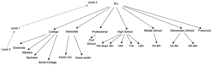
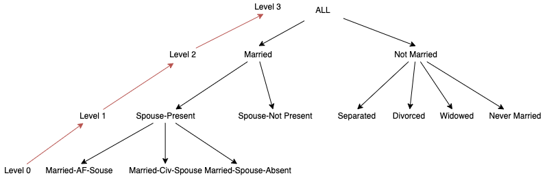
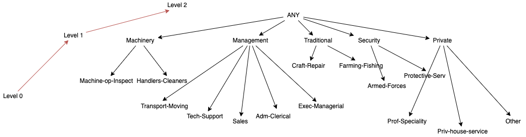
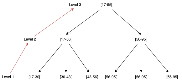
The remaining QIDs were transformed using an order-based hierarchy, as these are useful for string values that can be generalized in levels. For the creation of these it was considered their background semantics in the United States (e.g., education levels in US for the attribute education). These hierarchies can be found in Appendix D. One thing to note about these hierarchies is that its creation in ARX provided an unpleasant experience, due to how ARX represents levels visually. As such and given that to correctly create an order base hierarchy for the first time took approximately two hours, the authors of the report would like to describe a sample tutorial for the readers:
- Start by drawing the hierarchy on paper or in a digital platform that allows such, as it will be easier to understand the tree and translate it to ARX. We recommend the diagrams.net [20] platform as it is free, easy to use and open source;
- On ARX, select the attribute column to create the hierarchy and then select the “Create Hierarchy...” option under Edit tab; Also check the order-based hierarchy option since we are working with strings;
- You will be prompted with a view that has two sections: Order and Groups. The order section will be later used to order the appearance of the attribute values for the created levels. The groups section represents the levels of three, except for Level 0 and the highest tree level (i.e., ALL, ANY, *);
- Start by introducing the names described in Level 1 nodes. To do such, click on the first group, select the “Group” tab, apply the “Constant Value” aggregate function, set the name of the level node in “Function Parameter” and the number of descendant nodes as the “Size”. Do this until all level values have been described in ARX;
- Having all level nodes described, add upper levels if existing. You can do this by selecting the desired node, right-clicking it and selecting “Add new level”. You have now created a node which is on Level 2. You can now repeat the 4th step until all level nodes have been created;
- Upon reaching the level below the highest level, stop and order the attribute values so that these matches the described levels in ARX. You can get a better perspective of the tree when selecting next.
Coing Model Configuration
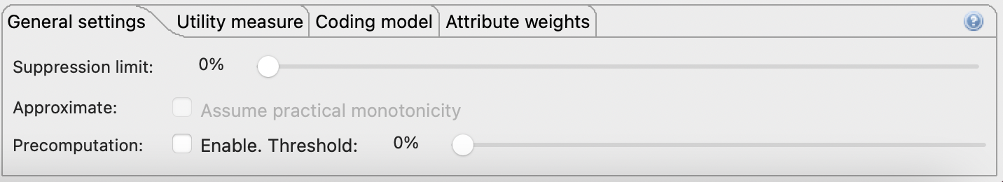
Some additional configurations can also be applied to increase or decrease both utility and privacy levels, by tunning the generalization and suppression parameters in ARX. As expected, if the generalization parameter is increased, the utility level will decrease as data is more general. On the other hand, by increasing the suppression parameter, the utility level may increase since instead of generalizing data, ARX will try to suppress potentially identifiable data.
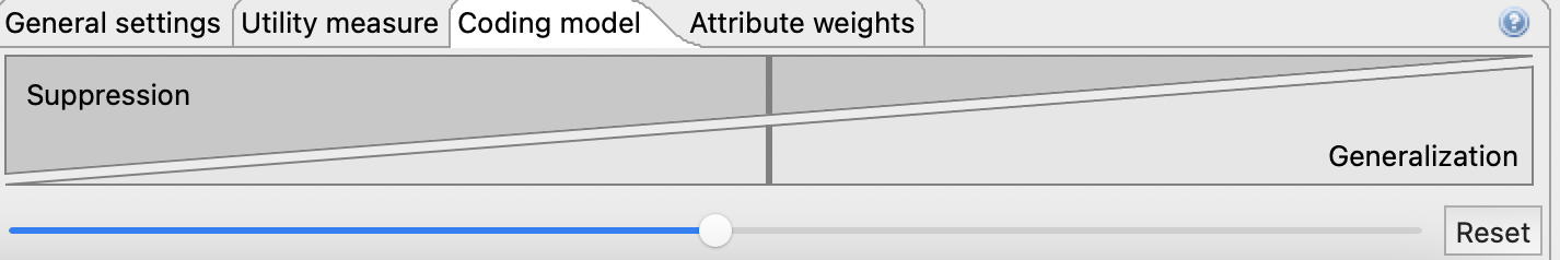
For now, these values will be kept balanced (50%/50%) for initial anonymization analysis and then refined to increase the utility of the dataset.
Preliminary Re-identification Risks Analysis
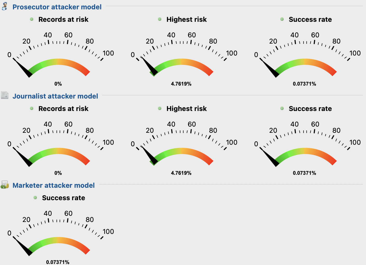
ARX offers a great view for analysis of re-identification risks based on the prosecutor, journalist and marketer attack models. These models try to identify a specific individual, any individual or as many individuals respectively, by calculating the size of equivalence classes (set of entries which QID attributes are equal [21]). Higher values of re-identification means that more and more dataset records are in risk of being identified, so a metric for privacy is to keep this as low as possible.
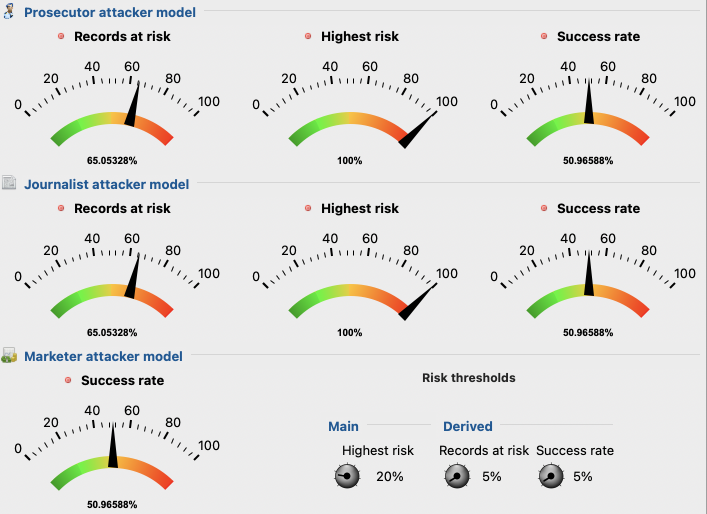
As seen above in Figure 7, the initials values of records at risk are high as no anonymization has been applied yet. This indicates that the privacy parameters set for the anonymization process will have to be adjusted, so that these values decrease.
Dataset Anonymization Analysis
This last chapter intends to present the reader the approaches taken by the report authors regarding the analysis of the anonymized dataset. First it will be necessary to briefly introduce the privacy models available that will target both QID and sensitive attributes during anonymization. Secondly, it will be presented the chosen privacy models and the reason for choosing these, as well as the applied privacy parameters. Then, on an iterative manner, the results obtained after anonymizing the dataset will be presented, evaluating the privacy and utility scores, comparing them to the original dataset goal. To conclude, it will be revealed if the goals for the anonymized dataset were accomplished, followed by some conclusions and future work for the dataset anonymization.
Privacy Models Review
The goal of privacy models is to protect re-identification of entities in the dataset, based on the prosecutor, journalist and marketer attack models [17]. These can be syntactic, in the way that data is transformed until a specific condition is met [22], and semantic, where data is transformed considering the dataset characteristics [17]. Popular syntactic models include:
- k-Anonymity, which form equivalence classes of k length. With these equivalence classes, anonymization operations such as generalization and suppression are applied, in order to anonymize data [17];
- l-Diversity, which also forms equivalence classes but grants that at least l distinct values are found for each sensitive attribute, protecting data of attributes disclosure [17];
- t-Closeness, which also protects data against attribute disclosure in equivalence classes, using the notion of Earth Movers Distance (EMD) value to calculate the difference between frequency distributions.
The biggest weakness of k-Anonymity is equivalence classes with sensitive attributes that lack diversity, that is, a set of dataset entries which QIDs attributes are equal and its sensitive attributes are equal or very similar. This lack of diversity allows attackers to perform homogeneity attacks, if the sensitive attributes are equal, or even background knowledge attacks by using external datasets and exploiting the dataset attributes semantics, since k-Anonymity does not consider it. To improve this lack of diversity, usually l-Diversity is combined with k-Anonymity, so that equivalences classes do not lack diversity.
Chosen Privacy Models
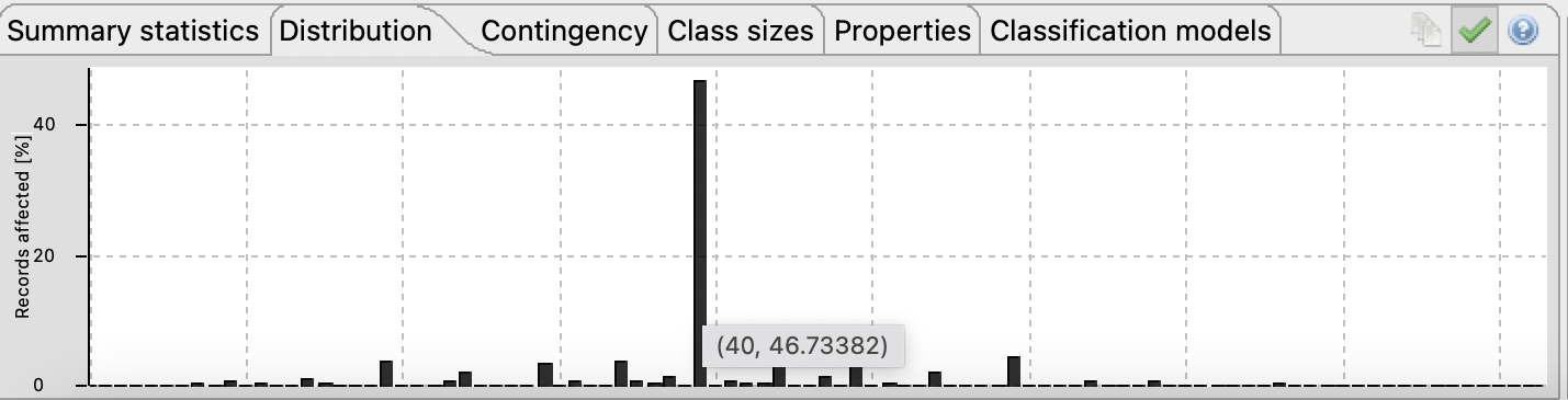
As described earlier, the dataset in context contains two sensitive attributes: hours per week and income. It is known that income only admits two values, which is an issue when using k-Anonymity since it lacks diversity in the values distribution. To fix this issue and in order to use k-Anonymity, it will be required to use l-Diversity for the income attribute. Upon further analysis it was found that the hours per week distribution may also be vulnerable to diversity attacks as the majority of values are represented by the casual working hours per week, which is 40. Given this, it will also be necessary to apply l-Diversity to this attribute.
Having elicited the privacy models to use, it is necessary to define values for the privacy parameters (k and l). Since k-Anonymity promotes generalization and higher k values tends for more generalized data, for a first iteration it will be assumed k=6 in order to attempt to reduce the re-identification risk. Regarding the l parameter it will be assumed l=2 since the income attribute cannot assume more than two values.
Once these values are defined the first iteration of anonymization can take place.
Analysis of Privacy Models Results
After the anonymization in ARX with the defined privacy models and parameters was executed, the first iteration values were analyzed. The first values analyzed were the attack models scores, to see if these had decreased. As depicted below in Figure 9, these values decreased by a lot, going from 65% to 0% in the prosecutor and journalist models. This was expected as the k value in use is high, increasing the generalization and thus privacy level of the dataset. However, despite solving the privacy level issue, 0% is a such a low score, meaning that the utility of the dataset must be very low.
Upon checking the information loss score in the Explore Results tab of ARX, it was noticed that about 56% of information was being loss. Jumping to the Analyze Utility tab it was noticed that QID attributes workclass, education and occupation had their anonymized distribution filled with the highest hierarchy level values (character '*'). This level of information loss was unacceptable for the dataset goal, so the k privacy parameter had to be refined.
Iteration 2: 3-Anonymity and 2-Diversity
Assuming that it was the k-Anonymity model causing so much loss of information, for a second analysis its value was reduced in half (k=3). However, when checking the attributes distribution, it was noticed that they were still fully generalized.
Iteration 3: 2-Anonymity and 2-Diversity
If it is really k-Anonymity the reason for such vague distributions, then setting its value to the lowest possible (2), the distributions would start being more diverse. Shockingly, it was not k-Anonymity causing such issues as the distributions were still fully generalized. What could be the root reason for so much generalization? Could it be the l-Diversity model? That would not make sense since this model focuses on sensitive attributes and promotes diversity. After performing a sanity check on the l value and noticing that it did not change anything for the distributions, the hierarchy levels of the target attributes were redefined. Unfortunately, no major changes occurred, meaning that either the QID attributes were incorrectly defined or the anonymized dataset really had no utility.
Iteration 4: 2-Anonymity, 2-Diversity and 5% Suppression Level
After losing hope of achieving the anonymized dataset goal and destroying and building back the dataset with new configurations, it was noticed that no suppression level was defined. This particular parameter allows defining the percentage of the number of outliers that can be removed from the dataset during the anonymization process.
Maybe this parameter will help as all the target attributes have missing values from the original dataset. For a brief analysis, this parameter was increased to 5%. Upon analysis of the distributions, it indeed had helped as now, the only distribution fully generalized was for the attribute education. Although implying suppression of data, this was excellent progress for meeting the anonymized goal.
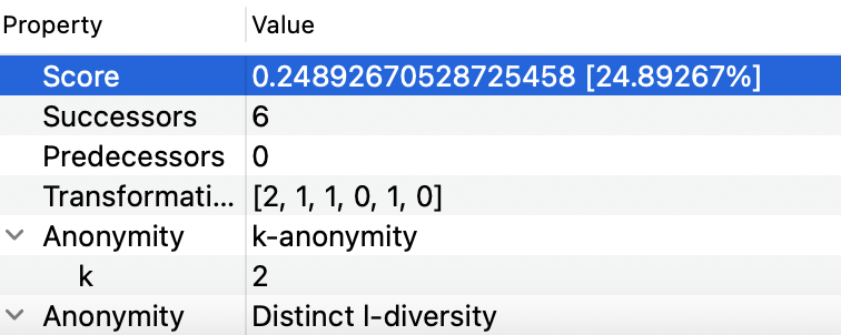
Iteration 5: 2-Anonymity, 2-Diversity and 12% Suppression
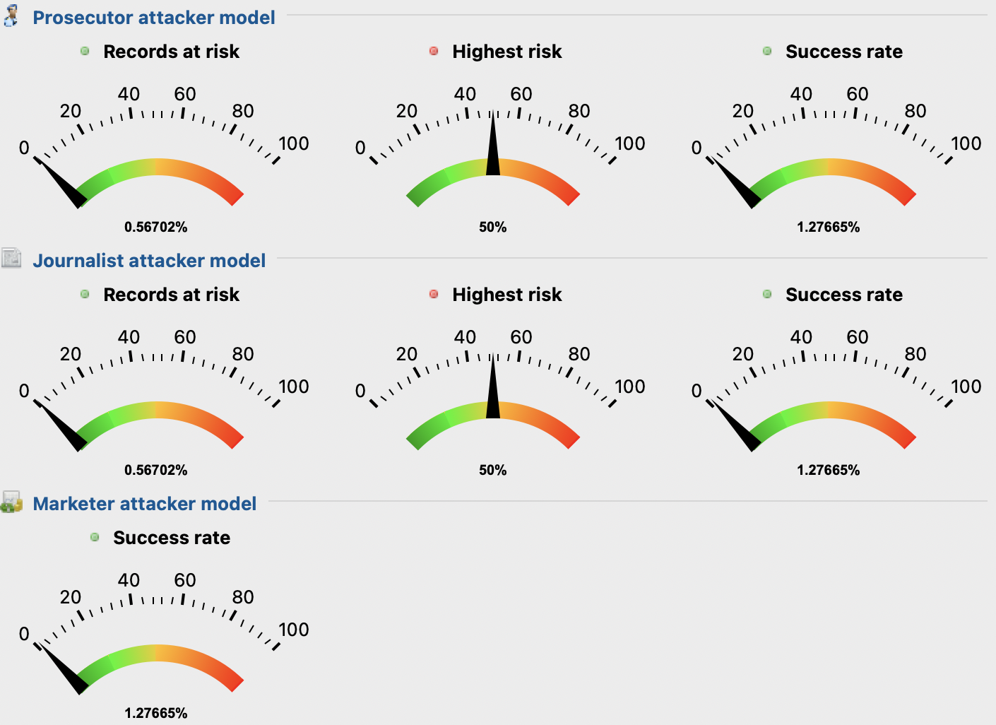
Knowing that the suppression level parameter was the key point for increasing the utility level, some tweaks here and there were applied. It was noticed that distributions were not fully generalized from the 12% interval. The team decided to stick with this value to prevent more information loss in terms of data suppression. By looking to Figure 11 and Figure 12 it can be noticed that the re-identification risks are low (close to 0.6%), with very low success rate (approx. 1.3%) and a not so big loss of information (~25%). The odd thing about this suppression level if increased to really high values (> = 80 %), the information loss score is 0%. This is very strange as the number of suppressed records is the same in both 12 and 80% anonymizations.
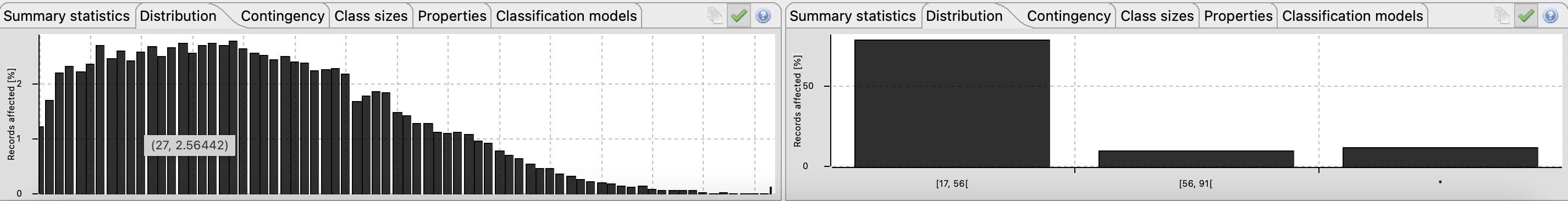
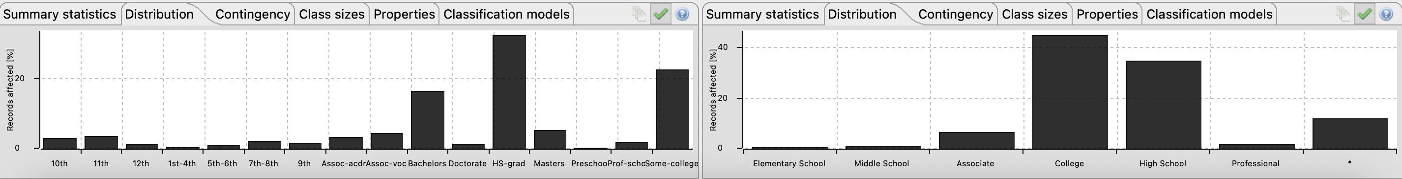
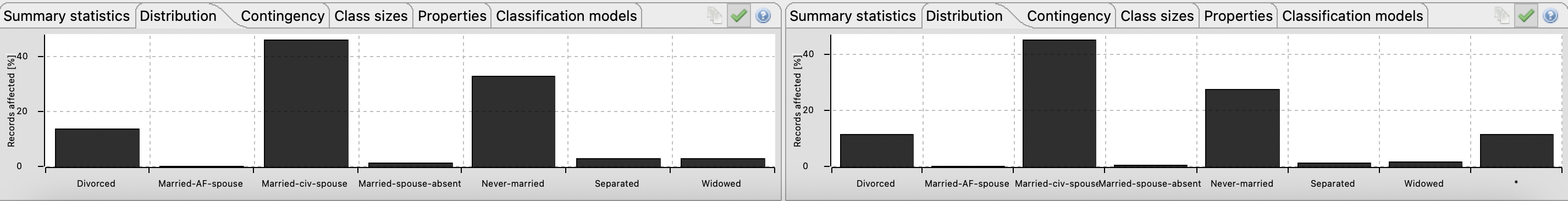
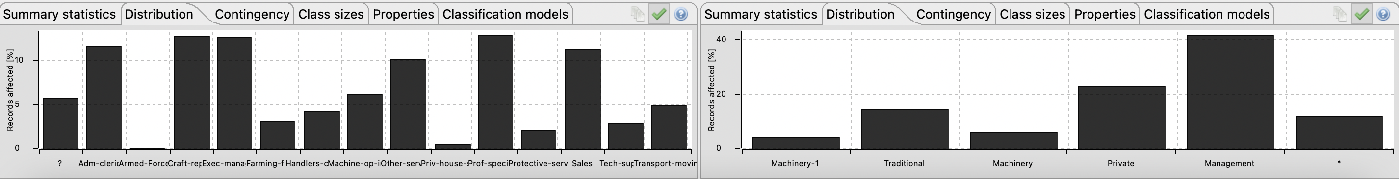
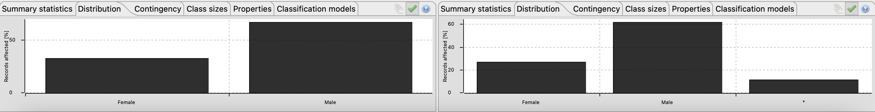
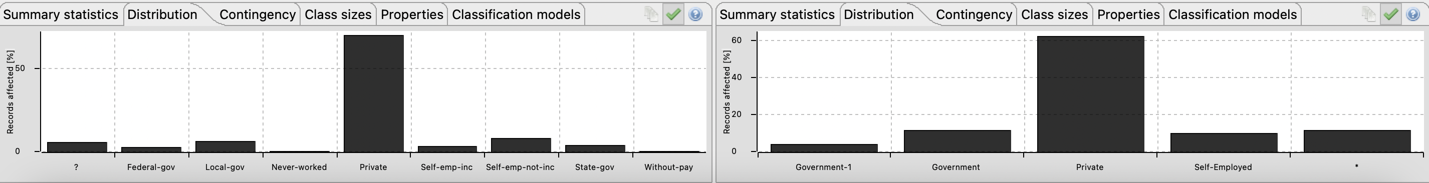
Furthermore, in Figure 13, 14, 15, 16, 17 and 18 present in Appendix B, it can be realized that the attributes distributions are not vague.
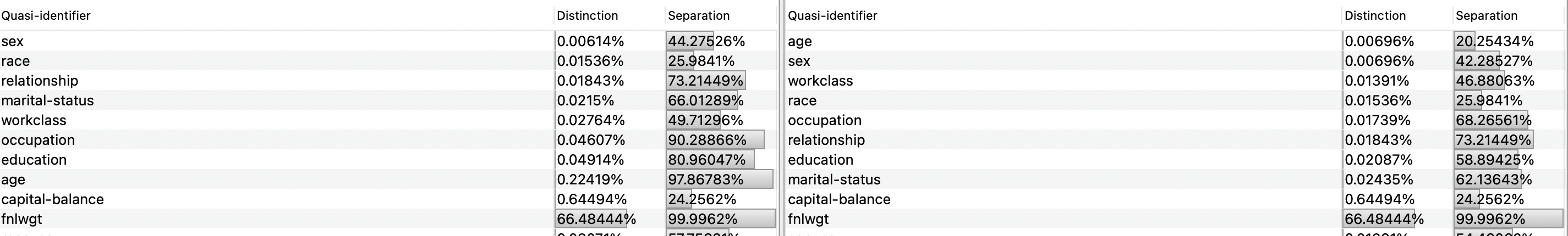
To conclude, Figure 19 present in Appendix C also proves that there was a decrease in the re-identification of entities in the dataset as the distinction and separation values of the attributed had decreased.
Conclusions and Future Work
In summary, it was set for the anonymized dataset goals that the utility levels had to be higher than 70%. This requirement is achieved as only 24% of information was lost. As for the privacy level, it was decided that this level had to be lower than 20%. Looking to the obtained re-identification scores, it is safe to say that this goal was met. Running the Kaggle notebook with the anonymized dataset, the prediction accuracy lowered to 0.80, 0.02 less than with the original dataset. With this value it is possible to conclude that the prediction goal was also met as 0.80 is higher than 0.738.
Regarding future work, the team suggests that other privacy models such as k-Map, δ-Presence are used for the QID attributes transformation, as well as other available privacy models for sensitive attributes. Additionally, it would also be cool to test other aggregate functions for the definition of hierarchy levels in ARX, as these may lead to different dataset transformations.
As a final note, the team has published the dataset sources, Kaggle, ARX and scripts source code publicly in a Github repository [23], so that the reader or other interested people can improve it, cite it or play with it.
References
[1] U. C. Bureau, ‘Census.gov’, Census.gov, 2021. https://www.census.gov/en.html (accessed Dec. 05, 2021).
[2] U. C. Bureau, ‘What We Do’, Census.gov, Nov. 18, 2021. https://www.census.gov/about/what.html (accessed Dec. 05, 2021).
[3] GOV.UK, CENSUS, ‘About the census’, Census 2021, 2021. https://census.gov.uk/about-the-census (accessed Dec. 01, 2021).
[4] UCI, ‘UCI Machine Learning Repository’, 2021. https://archive.ics.uci.edu/ml/index.php (accessed Dec. 01, 2021).
[5] UCI, ‘UCI Machine Learning Repository: About’, 2021. https://archive.ics.uci.edu/ml/about.html (accessed Dec. 01, 2021).
[6] C. Lemon, C. Zelazo, and M. Mulakaluri, ‘Predicting if income exceeds $50,000 per year based on 1994 US Census Data with Simple Classification Techniques’, 2018, [Online]. Available: https://cseweb.ucsd.edu/ jmcauley/cse190/reports/sp15/048.pdf
[7] A. Poncelet, ‘Adult Census Income’, 2016. https://kaggle.com/uciml/adult-census-income (accessed Dec. 02, 2021).
[8] K. El Eman and L. Arbuckle, Anonymizing Health Data. O’Reilly Media, Inc., 2013. [Online]. Available: https://www.oreilly.com/library/view/anonymizing-health-data/9781449363062/
[9] B. Akyuz, ‘ML101 k-NN’, Nov. 2021. https://kaggle.com/iambca/ml101-k-nn (accessed Dec. 05, 2021).
[10] O. Harrison, ‘Machine Learning Basics with the K-Nearest Neighbors Algorithm’, Medium, Jul. 14, 2019. https://towardsdatascience.com/machine-learning-basics-with-the-k-nearest-neighbors-algorithm-6a6e71d01761 (accessed Dec. 05, 2021).
[11] D. A. in K. A. R. P. E. W.-R. B. ARX, ‘Configuration | ARX - Data Anonymization Tool’, 2021. https://arx.deidentifier.org/anonymization-tool/configuration/ (accessed Dec. 03, 2021).
[12] ARX, ARX - Open Source Data Anonymization Software. 2021. Accessed: Dec. 04, 2021. [Online]. Available: https://github.com/arx-deidentifier/arx
[13] A. UCI, ‘Adult Dataset Source’, 2021. https://archive.ics.uci.edu/ml/machine-learning-databases/adult/ (accessed Dec. 03, 2021).
[14] E. Microsoft, ‘Microsoft Excel – Software de Folha de Cálculo | Microsoft 365’, 2021. https://www.microsoft.com/pt-pt/microsoft-365/excel (accessed Dec. 03, 2021).
[15] Python, ‘Welcome to Python.org’, Python.org, 2021. https://www.python.org/ (accessed Dec. 03, 2021).
[16] Pandas, ‘pandas - Python Data Analysis Library’, 2021. https://pandas.pydata.org/ (accessed Dec. 03, 2021).
[17] ARX, ‘Privacy models | ARX - Data Anonymization Tool’, 2021. https://arx.deidentifier.org/overview/privacy-criteria/ (accessed Dec. 04, 2021).
[18] M. Stewart, ‘Data Privacy in the Age of Big Data’, Medium, Jul. 29, 2020. https://towardsdatascience.com/data-privacy-in-the-age-of-big-data-c28405e15508 (accessed Dec. 04, 2021).
[19] W. Stallings, Information Privacy Engineering and Privacy by Design: Understanding privacy threats, technologies, and regulations, Original retail. 2020.
[20] diagrams, ‘Diagram Software and Flowchart Maker’, 2021. https://www.diagrams.net/ (accessed Dec. 05, 2021).
[21] ARX, ‘Utility analysis | ARX - Data Anonymization Tool’, 2021. https://arx.deidentifier.org/anonymization-tool/analysis/ (accessed Dec. 04, 2021).
[22] C. Clifton and T. Tassa, ‘On syntactic anonymity and differential privacy’, in 2013 IEEE 29th International Conference on Data Engineering Workshops (ICDEW), Brisbane, QLD, Apr. 2013, pp. 88–93. doi: 10.1109/ICDEW.2013.6547433.
[23] J. Freitas, Adult Dataset Anonymization Github Repository. 2021. Accessed: Dec. 05, 2021. [Online]. Available: https://github.com/freitzzz/trp-tp1
APPENDIX A – Description and Impacts of the Dataset Attributes
| Attribute | Description | Domain |
|---|---|---|
| age | Age of the individual, in a numerical format | [17, 90] |
| fnlwgt | An estimate number of individuals which the census believes that the data entry represents | [12285, 1484705] |
| income | A conditional string that states whether the user income is larger than 50k | <=50K, >50K |
| sex | Sex/Gender of the individual, in a binary string format | [Male, Female] |
| capital-gain | How much the net worth of the individual increased, in a numerical format | [0, 99999] |
| capital-loss | How much the net worth of the individual decreased, in a numerical format | [-4356, 0] |
| hours-per-week | The number of hours the individual works, in a numerical format | [1, 99] |
| education-num | Numerical number that represents the school degree in an index table | [1, 16] |
| Attribute | Description | Domain |
|---|---|---|
| workclass | Work class portrayed by the individual job, in a string format | State-gov, Self-emp-not-inc, Private, Federal-gov, Local-gov, ?, Self-emp-inc, Without-pay, Never-worked |
| race | Race of the individual, in a string format | White, Black, Asian-Pac-Islander, Amer-Indian-Eskimo, Other |
| marital-status | Marital status of the individual, in a string format | Never-married, Married-civ-spouse, Divorced, Married-spouse-absent, Separated, Married-AF-spouse, Widowed |
| relationship | An indicator of what the individual represents to its relatives, in a string format | Not-in-family, Husband, Wife, Own-child, Unmarried, Other-relative |
| Attribute | Description | Domain |
|---|---|---|
| education | Highest school degree of the individual, in a string format | Bachelors, HS-grad, 11th, Masters, 9th, Some-college, Assoc-acdm, Assoc-voc, 7th-8th, Doctorate, Prof-school, 5th-6th, 10th, 1st-4th, Preschool, 12th |
| occupation | Work field represented by the individual job, in a string format | Adm-clerical, Exec-managerial, Handlers-cleaners, Prof-specialty, Other-service, Sales, Craft-repair, Transport-moving, Farming-fishing, Machine-op-inspct, Tech-support, ?, Protective-serv, Armed-Forces, Priv-house-serv |
| native-country | The birth country of the individual | United-States, Cuba, Jamaica, India, ?, Mexico, South, Puerto-Rico, Honduras, England, Canada, Germany, Iran, Philippines, Italy, Poland, Columbia, Cambodia, Thailand, Ecuador, Laos, Taiwan, Haiti, Portugal, Dominican-Republic, El-Salvador, France, Guatemala, China, Japan, Yugoslavia, Peru, Outlying-US(Guam-USVI-etc), Scotland, Trinadad&Tobago, Greece, Nicaragua, Vietnam, Hong, Ireland, Hungary, Holand-Netherlands |
APPENDIX B – Original vs Anonymized Dataset Attributes Distribution
APPENDIX C – Original vs Anonymized Dataset Attributes Distinction and Separation Values
APPENDIX D – Created Order-based Hierarchy Trees