ematvey / visdom

A flexible tool for creating, organizing, and sharing visualizations of live, rich data. Supports Torch and Numpy.

Visdom

A flexible tool for creating, organizing, and sharing visualizations of live, rich data. Supports Torch and Numpy.

• Overview
• Concepts
• Setup
• Usage
• API
• To Do
• Contributing

Overview

Visdom aims to facilitate visualization of (remote) data with an emphasis on supporting scientific experimentation.

Broadcast visualizations of plots, images, and text for yourself and your collaborators.

Organize your visualization space programmatically or through the UI to create dashboards for live data, inspect results of experiments, or debug experimental code.

Concepts

Visdom has a simple set of features that can be composed for various use-cases.

Panes

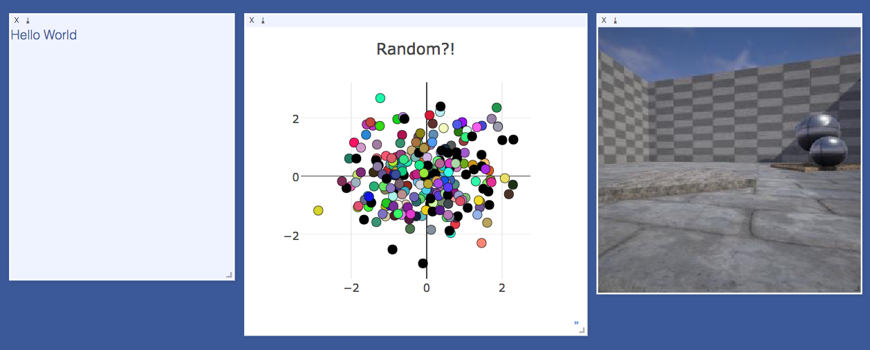
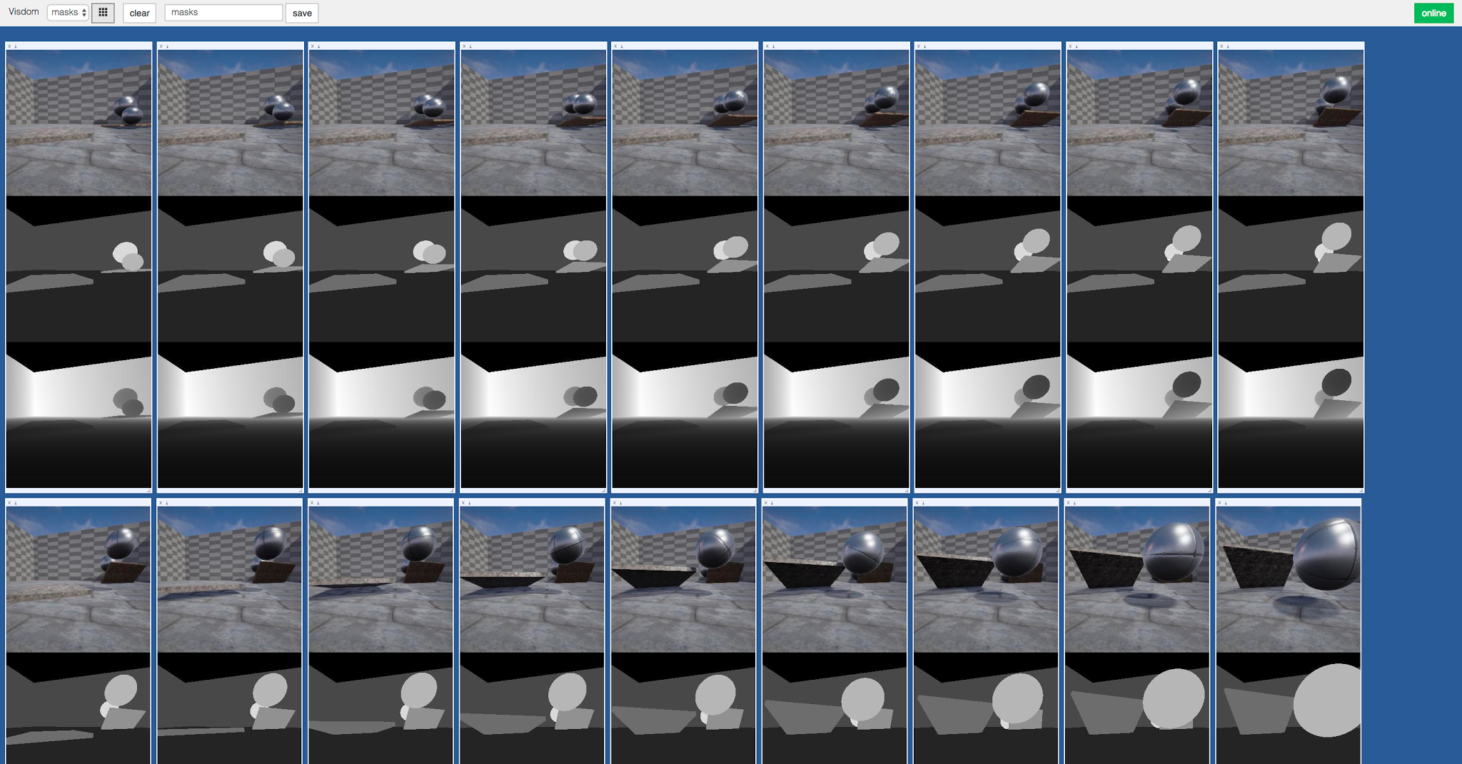
The UI begins as a blank slate -- you can populate it with plots, images, and text. These appear in panes that you can drag, drop, resize, and destroy. The panes live in envs and the state of envs is stored across sessions. You can download the content of panes -- including your plots in svg.

Tip: You can use the zoom of your browser to adjust the scale of the UI.

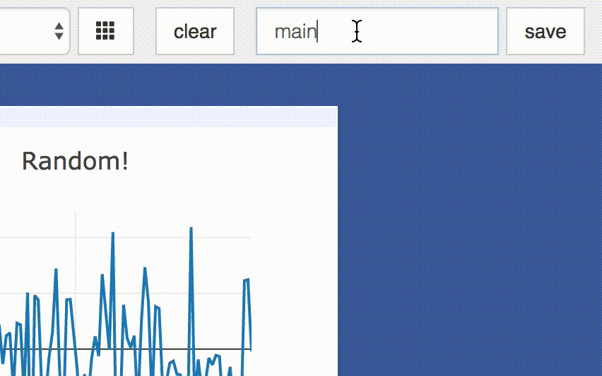
Environments

You can partition your visualization space with envs. By default, every user will have an env called main. New envs can be created in the UI or programmatically. The state of envs is chronically saved.

You can access a specific env via url: http://localhost.com:8097/env/main. If your server is hosted, you can share this url so others can see your visualizations too.

Managing Envs: Your envs are loaded at initialization of the server, by default from $HOME/.visdom/. Custom paths can be passed as a cmd-line argument. Envs are removed by deleting the corresponding .json file from the env dir.

State

Once you've created a few visualizations, state is maintained. The server automatically caches your visualizations -- if you reload the page, your visualizations reappear.

• Save: You can manually do so with the save button. This will serialize the env's state (to disk, in JSON), including window positions. You can save an env programmatically.
  This is helpful for more sophisticated visualizations in which configuration is meaningful, e.g. a data-rich demo, a model training dashboard, or systematic experimentation. This also makes them easy to share and reuse.

• Fork: If you enter a new env name, saving will create a new env -- effectively forking the previous env.

Filter

You can use the filter to dynamically sift through panes present in an env -- just provide a regular expression with which to match titles of pane you want to show. This can be helpful in use cases involving an env with many panes e.g. when systematically checking experimental results.

Setup

Requires Python 2.7/3 (and optionally Torch7)

# Install Python server and client
pip install visdom

# Install Torch client
luarocks install visdom

Launch

Start the server (probably in a screen or tmux) :

python -m visdom.server

Visdom now can be accessed by going to http://localhost:8097 in your browser, or your own host address if specified.

If the above does not work, try using an SSH tunnel to your server by adding the following line to your local ~/.ssh/config: LocalForward 127.0.0.1:8097 127.0.0.1:8097.

Python example

import visdom
import numpy as np
vis = visdom.Visdom()
vis.text('Hello, world!')
vis.image(np.ones((3, 10, 10)))

Torch example

require 'image'
vis = require 'visdom'()
vis:text{text = 'Hello, world!'}
vis:image{img = image.fabio()}

Some users have reported issues when connecting Lua clients to the Visdom server. A potential work-around may be to switch off IPv6:

vis = require 'visdom'()
vis.ipv6 = false  -- switches off IPv6
vis:text{text = 'Hello, world!'}

Demos

python example/demo.py
th example/demo1.lua
th example/demo2.lua

API

For a quick introduction into the capabilities of visdom, have a look at the example directory, or read the details below.

Basics

Visdom offers the following basic visualization functions:

• vis.image : image
• vis.images : list of images
• vis.text : arbitrary HTML
• vis.video : videos
• vis.svg : SVG object
• vis.save : serialize state server-side

Plotting

We have wrapped several common plot types to make creating basic visualizations easily. These visualizations are powered by Plotly.

The following API is currently supported:

• vis.scatter : 2D or 3D scatter plots
• vis.line : line plots
• vis.updateTrace : update existing line/scatter plots
• vis.stem : stem plots
• vis.heatmap : heatmap plots
• vis.bar : bar graphs
• vis.histogram: histograms
• vis.boxplot : boxplots
• vis.surf : surface plots
• vis.contour : contour plots
• vis.quiver : quiver plots
• vis.mesh : mesh plots

Generic Plots

Note that the server API adheres to the Plotly convention of data and layout objects, such that you can produce your own arbitrary Plotly visualizations:

import visdom
vis = visdom.Visdom()

trace = dict(x=[1,2,3], y=[4,5,6], marker={'color': 'red', 'symbol': 104, 'size': "10"},
                    mode="markers+lines",  text=["one","two","three"], name='1st Trace')
layout=dict(title="First Plot", xaxis={'title':'x1'}, yaxis={'title':'x2'})

vis._send({'data': [trace], 'layout': layout, 'win': 'mywin'})

Details

vis.image

This function draws an img. It takes as input an CxHxW tensor img that contains the image.

The following options are supported:

• options.jpgquality: JPG quality (number 0-100; default = 100)
• options.caption: Caption for the image

vis.images

This function draws a list of images. It takes an input B x C x H x W tensor or a list of images all of the same size. It makes a grid of images of size (B / nrow, nrow).

The following arguments and options are supported:

• nrow: Number of images in a row
• padding: Padding around the image, equal padding around all 4 sides
• options.jpgquality: JPG quality (number 0-100; default = 100)
• options.caption: Caption for the image

vis.text

This function prints text in a box. You can use this to embed arbitrary HTML. It takes as input a text string. No specific options are currently supported.

vis.video

This function plays a video. It takes as input the filename of the video videofile or a LxCxHxW-sized tensor (in Lua) or a or a LxHxWxC-sized tensor (in Python) containing all the frames of the video as input. The function does not support any plot-specific options.

The following options are supported:

• options.fps: FPS for the video (integer > 0; default = 25)

Note: Using tensor input requires that ffmpeg is installed and working. Your ability to play video may depend on the browser you use: your browser has to support the Theano codec in an OGG container (Chrome supports this).

vis.svg

This function draws an SVG object. It takes as input a SVG string svgstr or the name of an SVG file svgfile. The function does not support any specific options.

Simple Plots

Further details on the wrapped plotting functions are given below.

The exact inputs into the plotting functions vary, although most of them take as input a tensor X than contains the data and an (optional) tensor Y that contains optional data variables (such as labels or timestamps). All plotting functions take as input an optional win that can be used to plot into a specific window; each plotting function also returns the win of the window it plotted in. One can also specify the env to which the visualization should be added.

vis.scatter

This function draws a 2D or 3D scatter plot. It takes as input an Nx2 or Nx3 tensor X that specifies the locations of the N points in the scatter plot. An optional N tensor Y containing discrete labels that range between 1 and K can be specified as well -- the labels will be reflected in the colors of the markers. The following options are supported:

• options.colormap : colormap (string; default = 'Viridis')
• options.markersymbol: marker symbol (string; default = 'dot')
• options.markersize : marker size (number; default = '10')
• options.markercolor : color per marker. (torch.*Tensor; default = nil)
• options.legend : table containing legend names

options.markercolor is a Tensor with Integer values. The tensor can be of size N or N x 3 or K or K x 3.

• Tensor of size N: Single intensity value per data point. 0 = black, 255 = red
• Tensor of size N x 3: Red, Green and Blue intensities per data point. 0,0,0 = black, 255,255,255 = white
• Tensor of size K and K x 3: Instead of having a unique color per data point, the same color is shared for all points of a particular label.

vis.line

This function draws a line plot. It takes as input an N or NxM tensor Y that specifies the values of the M lines (that connect N points) to plot. It also takes an optional X tensor that specifies the corresponding x-axis values; X can be an N tensor (in which case all lines will share the same x-axis values) or have the same size as Y.

The following options are supported:

• options.fillarea : fill area below line (boolean)
• options.colormap : colormap (string; default = 'Viridis')
• options.markers : show markers (boolean; default = false)
• options.markersymbol: marker symbol (string; default = 'dot')
• options.markersize : marker size (number; default = '10')
• options.legend : table containing legend names

vis.updateTrace

This function allows updating of data for extant line or scatter plots.

It is up to the user to specify name of an existing trace if they want to add to it, and a new name if they want to add a trace to the plot. By default, if no legend is specified at time of first creation, the name is the index of the line in the legend.

If no name is specified, all traces should be updated. Trace update data that is all NaN is ignored; this can be used for masking update.

The append parameter determines if the update data should be appended to or replaces existing data.

There are no options because they are assumed to be inherited from the specified plot.

vis.stem

This function draws a stem plot. It takes as input an N or NxM tensor X that specifies the values of the N points in the M time series. An optional N or NxM tensor Y containing timestamps can be specified as well; if Y is an N tensor then all M time series are assumed to have the same timestamps.

The following options are supported:

• options.colormap: colormap (string; default = 'Viridis')
• options.legend : table containing legend names

vis.heatmap

This function draws a heatmap. It takes as input an NxM tensor X that specifies the value at each location in the heatmap.

The following options are supported:

• options.colormap : colormap (string; default = 'Viridis')
• options.xmin : clip minimum value (number; default = X:min())
• options.xmax : clip maximum value (number; default = X:max())
• options.columnnames: table containing x-axis labels
• options.rownames : table containing y-axis labels

vis.bar

This function draws a regular, stacked, or grouped bar plot. It takes as input an N or NxM tensor X that specifies the height of each of the bars. If X contains M columns, the values corresponding to each row are either stacked or grouped (depending on how options.stacked is set). In addition to X, an (optional) N tensor Y can be specified that contains the corresponding x-axis values.

The following plot-specific options are currently supported:

• options.columnnames: table containing x-axis labels
• options.stacked : stack multiple columns in X
• options.legend : table containing legend labels

vis.histogram

This function draws a histogram of the specified data. It takes as input an N tensor X that specifies the data of which to construct the histogram.

The following plot-specific options are currently supported:

• options.numbins: number of bins (number; default = 30)

vis.boxplot

This function draws boxplots of the specified data. It takes as input an N or an NxM tensor X that specifies the N data values of which to construct the M boxplots.

The following plot-specific options are currently supported:

• options.legend: labels for each of the columns in X

vis.surf

This function draws a surface plot. It takes as input an NxM tensor X that specifies the value at each location in the surface plot.

The following options are supported:

• options.colormap: colormap (string; default = 'Viridis')
• options.xmin : clip minimum value (number; default = X:min())
• options.xmax : clip maximum value (number; default = X:max())

vis.contour

This function draws a contour plot. It takes as input an NxM tensor X that specifies the value at each location in the contour plot.

The following options are supported:

• options.colormap: colormap (string; default = 'Viridis')
• options.xmin : clip minimum value (number; default = X:min())
• options.xmax : clip maximum value (number; default = X:max())

vis.quiver

This function draws a quiver plot in which the direction and length of the arrows is determined by the NxM tensors X and Y. Two optional NxM tensors gridX and gridY can be provided that specify the offsets of the arrows; by default, the arrows will be done on a regular grid.

The following options are supported:

• options.normalize: length of longest arrows (number)
• options.arrowheads: show arrow heads (boolean; default = true)

vis.mesh

This function draws a mesh plot from a set of vertices defined in an Nx2 or Nx3 matrix X, and polygons defined in an optional Mx2 or Mx3 matrix Y.

The following options are supported:

• options.color: color (string)
• options.opacity: opacity of polygons (number between 0 and 1)

Customizing plots

The plotting functions take an optional options table as input that can be used to change (generic or plot-specific) properties of the plots. All input arguments are specified in a single table; the input arguments are matches based on the keys they have in the input table.

The following options are generic in the sense that they are the same for all visualizations (except plot.image and plot.text):

• options.title : figure title
• options.width : figure width
• options.height : figure height
• options.showlegend : show legend (true or false)
• options.xtype : type of x-axis ('linear' or 'log')
• options.xlabel : label of x-axis
• options.xtick : show ticks on x-axis (boolean)
• options.xtickmin : first tick on x-axis (number)
• options.xtickmax : last tick on x-axis (number)
• options.xtickvals : locations of ticks on x-axis (table of numbers)
• options.xticklabels : ticks labels on x-axis (table of strings)
• options.xtickstep : distances between ticks on x-axis (number)
• options.ytype : type of y-axis ('linear' or 'log')
• options.ylabel : label of y-axis
• options.ytick : show ticks on y-axis (boolean)
• options.ytickmin : first tick on y-axis (number)
• options.ytickmax : last tick on y-axis (number)
• options.ytickvals : locations of ticks on y-axis (table of numbers)
• options.yticklabels : ticks labels on y-axis (table of strings)
• options.ytickstep : distances between ticks on y-axis (number)
• options.marginleft : left margin (in pixels)
• options.marginright : right margin (in pixels)
• options.margintop : top margin (in pixels)
• options.marginbottom: bottom margin (in pixels)

The other options are visualization-specific, and are described in the documentation of the functions.

To Do

• Command line tool for easy systematic plotting from live logs.
• Filtering through panes with regex by title (or meta field)
• Compiling react by python server at runtime

Contributing

See guidelines for contributing here.

Acknowledgments

Visdom was inspired by tools like display and relies on Plotly as a plotting front-end.