Corona timelapse

[Rodrigo Hernangómez]

Germany has lifted the travel restrictions for all regions upon the mildness of the omicron variant.

Since this renders the site quite uninteresting, I suggest to collect all the risk levels for each country over time so that some nice visualization can be implemented. This can be broken down into two tasks:

1. The creation of a table with all the risk levels over time, assigned to @rodrihgh
2. The (probably R-based) visualization, assigned to @dieghernan

My plan for the table is to have it as a CSV with the following structure:

	COUNTRY_ISO_CODE_A	COUNTRY_ISO_CODE_B	...
date_1	risk_code1.A	risk_code1.B	...
date_2	risk_code2.A	risk_code2.B	...
...	...	...	...

[Rodrigo Hernangómez]

I have created a table with dummy risk level codes in case you want to start playing around with the visualization, @dieghernan

https://github.com/dieghernan/RKI-Corona-Atlas/blob/dev/timelapse/mockup.csv

[Diego H.]

An initial attempt (really basic, it can be largely improved):

download.file("https://raw.githubusercontent.com/dieghernan/RKI-Corona-Atlas/dev/timelapse/mockup.csv",
              "mockup.csv")
download.file("https://raw.githubusercontent.com/dieghernan/RKI-Corona-Atlas/master/assets/geo/country_shapes.geojson",
              "country_shapes.geojson")


library(tidyverse)
library(sf)
#> Linking to GEOS 3.9.1, GDAL 3.2.1, PROJ 7.2.1; sf_use_s2() is TRUE
library(gganimate)

evo <- read_csv("mockup.csv")
#> New names:
#> * `` -> ...1
#> Rows: 52 Columns: 199
#> -- Column specification --------------------------------------------------------
#> Delimiter: ","
#> dbl  (198): AFG, AGO, ALB, AND, ARE, ARG, ARM, ATG, AUS, AUT, AZE, BDI, BEL,...
#> date   (1): ...1
#> 
#> i Use `spec()` to retrieve the full column specification for this data.
#> i Specify the column types or set `show_col_types = FALSE` to quiet this message.
shape <- st_read("country_shapes.geojson")
#> Reading layer `country_shapes' from data source 
#>   `C:\Users\diego\AppData\Local\Temp\RtmpiI3gt8\reprex-4e034ac1e65-vivid-eider\country_shapes.geojson' 
#>   using driver `GeoJSON'
#> Simple feature collection with 198 features and 1 field
#> Geometry type: MULTIPOLYGON
#> Dimension:     XY
#> Bounding box:  xmin: -180 ymin: -59.51912 xmax: 180 ymax: 83.65187
#> Geodetic CRS:  WGS 84
shape <- st_transform(shape, "+proj=robin")

# Modify evo
n <- names(evo)
n[1] <- "date"
names(evo) <- n
evo2 <- evo %>%
  pivot_longer(!date, names_to = "ISO3_CODE")


# Background
bck <- st_graticule() %>%
  st_bbox() %>%
  st_as_sfc() %>%
  st_transform(3857) %>%
  st_segmentize(500000) %>%
  st_transform(st_crs(shape))


shapeend <- shape %>% left_join(evo2) %>%
  arrange(date, ISO3_CODE)
#> Joining, by = "ISO3_CODE"

shapeend$value <- as.factor(shapeend$value)


DEU <- shape %>% filter(ISO3_CODE=="DEU")


files <- str_c("./ta_anima/D", str_pad(seq_len(nrow(evo))
  , 3, "left", "0"), ".png")


dates <- as.character(evo$date)

 
for (i in seq_len(nrow(evo))){
datloop <- dates[i]
ggplot(shapeend %>% filter(date ==datloop)) +
  geom_sf(data=bck, fill="lightblue", alpha=0.4) +
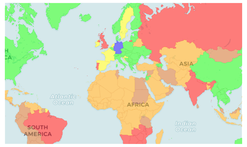
  geom_sf(aes(fill=value), show.legend = FALSE, size=0.01) +
  geom_sf(data=DEU, fill="blue", size = 0.01) +
  scale_fill_manual(values = c("#00FF00", "red", "chocolate", "orange", "yellow")) +
  theme_void() +
  theme(plot.background = element_rect(fill="white", color=NA)) +
  labs(
    title = "Corona Atlas",
    subtitle = datloop,
    caption = "Data: Robert Koch Institut",
    fill = ""
  )

ggsave(files[i], width = 1000, height = 700, dpi=300, units = "px")
}

library(gifski)


gifski(files, "tmx_covid.gif", width = 1000, height = 700, loop = FALSE, delay = 0.5)
#> [1] "C:\\Users\\diego\\AppData\\Local\\Temp\\RtmpiI3gt8\\reprex-4e034ac1e65-vivid-eider\\tmx_covid.gif"

^{Created on 2022-03-06 by the reprex package (v2.0.1)}

[Rodrigo Hernangómez]

I have just added the actual data in dev/timelapse/risk_date_countries.csv.

Here I have included the risk levels 3 (Risk area) and 4 (Partial risk area, i.e., countries which had some regions under moderate risk and some with no risk).

These were valid from Apr21 to Aug21. After that, the category "risk area" disappeared and the RKI used only"high-risk area" and "virus variant area".

[Diego H.]

FYI I can produce also mp4 files ;)

A version with transitions:

# # https://github.com/dieghernan/RKI-Corona-Atlas/blob/dev/timelapse/risk_date_countries.csv
#
# download.file("https://raw.githubusercontent.com/dieghernan/RKI-Corona-Atlas/dev/timelapse/risk_date_countries.csv",
#               "mockup.csv")
# download.file("https://raw.githubusercontent.com/dieghernan/RKI-Corona-Atlas/master/assets/geo/country_shapes.geojson",
#               "country_shapes.geojson")


library(tidyverse)
library(sf)

# Import
evo <- read_csv("mockup.csv")
shape <- st_read("country_shapes.geojson") %>%
  st_transform("+proj=robin")

# Shapes
deu <- shape %>% filter(ISO3_CODE == "DEU")
world <- shape %>% filter(ISO3_CODE != "DEU")


# Modify evo
n <- names(evo)
n[1] <- "date"
names(evo) <- n


a <- evo[1, ]

a <- a %>% select(-date)


paste0(sort(unique(as.vector(t(a)))), collapse = ",")

values <- lapply(1:nrow(evo), function(x) {
  a <- evo[x, ]

  a <- a %>% select(-date)

  s <- sort(unique(as.vector(t(a))))
  s <- s[s != 5]
  codes <- paste0(s, collapse = ",")
  return(codes)
})

analisis <- evo %>%
  select(date) %>%
  mutate(values = unlist(values))


evo2 <- evo %>%
  pivot_longer(!date, names_to = "ISO3_CODE")


# Background
bck <- st_graticule() %>%
  st_bbox() %>%
  st_as_sfc() %>%
  st_transform(3857) %>%
  st_segmentize(500000) %>%
  st_transform(st_crs(shape))


# Loop
alldates <- unique(sort(evo2$date))
files <- str_c("./covid/D", str_pad(
  seq_len(length(alldates)),
  3, "left", "0"
), ".png")

# i = 1
#
# alldates <- alldates[1]

for (i in seq_len(length(alldates))) {
  d <- alldates[i]
  message("Date is ", as.character(d))

  # Map

  dat <- evo2 %>% filter(date == d)

  shapedat <- world %>% left_join(dat)


  # levels
  low <- shapedat %>% filter(value == 0)
  partial <- shapedat %>% filter(value == 4)
  risk <- shapedat %>% filter(value == 3)
  high <- shapedat %>% filter(value == 2)
  concern <- shapedat %>% filter(value == 1)
  rest <- shapedat %>% filter(!value %in% c(0:4))

  # Mock level for legend
  low$value <- as.factor(low$value)

  levels(low$value) <- c(
    "Not risk area",
    "Risk Area (Partial)",
    "Risk Area",
    "High risk area",
    "Variant of concern",
    "Germany"
  )

  # Base map
  base <- ggplot() +
    geom_sf(data = bck, fill = "lightblue", alpha = 0.4) +
    theme_void() +
    theme(
      plot.background = element_rect(fill = "white", color = NA),
      text = element_text(family = "roboto"),
      plot.title = element_text(hjust = .5, face = "bold", size = 15),
      plot.subtitle = element_text(hjust = .5, size = 5, face = "italic"),
      plot.caption = element_text(size = 5),
      legend.text = element_text(size = 4)
    ) +
    labs(
      title = "Corona Atlas",
      subtitle = as.character(d),
      caption = "Data: Robert Koch Institut ",
      fill = ""
    ) +
    geom_sf(data = deu, fill = "blue", size = 0.01)


  if (nrow(low) > 1) {
    base <- base +
      geom_sf(data = low, aes(fill = value), size = 0.01) +
      scale_fill_manual(
        values = c(
          "#00FF00",
          "yellow",
          "orange",
          "red",
          "chocolate",
          "blue"
        ),
        drop = FALSE
      ) +
      guides(fill = guide_legend(
        keywidth = 0.4,
        keyheight = .4
      ))
  }
  if (nrow(partial) > 1) {
    base <- base +
      geom_sf(data = partial, size = 0.01, fill = "yellow")
  }


  if (nrow(risk) > 1) {
    base <- base +
      geom_sf(data = risk, size = 0.01, fill = "orange")
  }


  if (nrow(high) > 1) {
    base <- base +
      geom_sf(data = high, size = 0.01, fill = "red")
  }



  if (nrow(concern) > 1) {
    base <- base +
      geom_sf(data = concern, size = 0.01, fill = "chocolate")
  }

  if (nrow(rest) > 1) {
    base <- base +
      geom_sf(data = rest, size = 0.01, fill = "grey70")
  }


  file <- files[i]

  ggsave(files[i], base, width = 1000, height = 700, dpi = 300, units = "px")
}



# Animation
library(magick)
library(dplyr)

allf <- list.files("covid", pattern = ".png$", full.names = TRUE)

imgs <- image_read(allf)

anim <- imgs %>%
  image_morph()

image_write_gif(anim, "covid.gif",
  delay =
    1 / 15,
  progress = TRUE
)

Pure timelapse

[Rodrigo Hernangómez]

Very nice! I would suggest swapping the colors for "High risk area" and "Variant of concern", as we also ended up doing in the site:

[Diego H.]

Would do, also I would add Antarctica even though we don't have data (the world map is just incomplete without it, hurt my eyes)

[Rodrigo Hernangómez]

Another action point to me: Retrieve older versions of the RKI site by scraping together with a wayback machine.

See for instance sangaline/scrapy-wayback-machine@22d525d

[Diego H.]

Got this so far.

@rodrihgh if we set a method to update https://github.com/dieghernan/RKI-Corona-Atlas/blob/dev/timelapse/risk_date_countries.csv and we deploy it to master branch, the gif can be created automatically using the gh-action

[Diego H.]

Note that #19 updated the gh-actions, in case you need also to do any modification. It could be a good idea to merge/rebase your branch

[Diego H.]

It is set now on gif branch, check it