Unsupervised Point Cloud Reconstruction for Classific Feature Learning
Introduction
Can unsupervised point cloud reconstruction extract features suitable for classification?
This work aims to show whether learning a unsupervised point cloud reconstruction task, for example FoldingNet, is able to extract features performing well in classification. We do all experiments under the framework of FoldingNet.
Details for FoldingNet see FoldingNet: Point Cloud Auto-encoder via Deep Grid Deformation (https://arxiv.org/abs/1712.07262).
We also tried to use DGCNN as encoder. DGCNN provides two type of networks, one for classification and one for segmentation. We use "DGCNN_Cls" to denote network for classification and "DGCNN_Seg" for segmentation. For both network, we adopt the feature extraction part as encoder in FoldingNet.
Experimental results show that better reconstruction performance do not correspond with better classfication accuracy of linear SVM classifier. Feature which good at classfication contains more nonobjective information, losing the ability to reconstruct detailedly. However, it is only this nonobjective information that is capable to capture the high level characteristic of its belonging category and thus make a great contribution in classfication task.
The key contributions of this work are as follows:
- We provide a pytorch reimplementation for FoldingNet.
- We also use source points for decoder from sphere surface and gaussian distribution. Results show that source points from sphere surface can reconstruct better.
- We do experiments using DGCNN as encoder and provide the classification performance for linear SVM classifier. The transfer dataset performance is better than the state-of-the-art unsupervised methods. We also train our best unsupervised model supervisedly, our unsupervised results still win out.
- We illustrate that better reconstruction results do not correspond with better feature for classfication.
If you find this work useful, please cite:
@article{tao2020,
      Author = {An Tao},
      Title = {Unsupervised Point Cloud Reconstruction for Classific Feature Learning},
      Journal = {https://github.com/AnTao97/UnsupervisedPointCloudReconstruction},
      Year = {2020}
}
For more our works on point cloud feature learning, see this repo.
Requirements
- Python 3.7
- PyTorch 1.2
- CUDA 10.0
- Package: glob, h5py, tensorflow, tensorboard, tensorboardX and sklearn
Download datasets
Download the HDF5 format datasets (where each shape is sampled 2,048 points uniformly):
- ShapeNetCore.v2 (0.98G) [TsinghuaCloud] [BaiduDisk]
- ModelNet40 (194M) [TsinghuaCloud] [BaiduDisk]
You can find more details about the above datasets in this repo.
Experiment settings
To evaluate the quality of extracted features, we use ShapeNetCore.v2 dataset to both train the FoldingNet auto-encoder and a linear SVM classifier. Specifically, we train the linear SVM classifier on ShapeNetCore.v2 dataset using the features (latent representations) obtained from the auto-encoder, while training the autoencoder from the ShapeNetCore.v2 dataset with 278 epoches.
For transfer performance, we train the linear SVM classifier on ModelNet 40 dataset using the features (latent representations) obtained from the same auto-encoder trained from the ShapeNetCore.v2 dataset.
FoldingNet has demonstrated that a 2D plane grid can be gradually folded into a meaningful point cloud. However, can uniformly sampled points from surface of sphere gradually turn into a meaningful point cloud? This is reasonable because 3D point clouds are actually sampled from surface of an object. We generate source points from surface of sphere using farthest point sampling algorithm.
A cloud of points corresponding to a shape can also be thought of as samples from a distribution that corresponds to the surface of this shape. Thus the goal for reconstruction task is to train a model which is able to transform source distribution, for example gaussian distribution, into the distribution corresponds to the surface of this shape. In this work we also try to use source points for decoder sampled from gaussian distribution N(0, I). However, it's worth noting that there is no relationship among x, y and z axises for points sampled from gaussian distribution, while for points from both plane grid and sphere surfance the relationship exists. Also because points sampled from gaussian distribution are i.i.d., there is no relationship among all points.
In all experiments, we follow the training scheme of FoldingNet.
Note that:
- Other than using the modified Chamfer distance in FoldingNet paper, we adopt the original Chamfer distance proposed by A Point Set Generation Network for 3D Object Reconstruction from a Single Image:
- To use the local covariance proposed in FoldingNet paper, pleanse comment line 49 and uncomment line 50 in
model.py. See this issue for detailed information.
To train the network, run
python main.py --exp_name <exp name> --dataset_root <root directory for datasets> --encoder <foldnet | dgcnn_cls | dgcnn_seg> --k <16 | 20 | 40> --shape <plane | sphere | gaussian> --dataset shapenetcorev2 --gpu <gpu ids>
You can download our already trained models from [TsinghuaCloud] or [BaiduDisk] and place them under snapshot/.
To evaluate the performance of a given trained model, run
python main.py --eval --model_path <model path> --dataset_root <root directory for datasets> --encoder <foldnet | dgcnn_cls | dgcnn_seg> --k <16 | 20 | 40> --shape <plane | sphere | gaussian> --dataset <shapenetcorev2 | modelnet40> --batch_size 4 --gpu <gpu ids>
Use --no_cuda if you want to run in CPU.
To visulize the reconstruction performance, run
python visualization.py --dataset_root <root directory for datasets> --dataset <modelnet40 | shapenetcorev2> --item=<index for data> --split <train | test> --encoder <foldnet | dgcnn_cls | dgcnn_seg> --k <16 | 20 | 40> --shape <plane | sphere | gaussian> --model_path=snapshot/<exp name>/models --draw_original --draw_source_points
Our script generates XML files and you are required to use Mitsuba to render them.
To use Tensorboard, run
tensorboard --logdir tensorboard --bind_all
You can find the Tensorboard records under tensorboard/.
Classification accuracy of linear SVM classifier
Results with different settings
| Encoder | K | Epochs | Shape | ShapeNetCore.v2 | ModelNet40 | |
|---|---|---|---|---|---|---|
| FoldingNet paper | Original | 16 | 278 | Plane | Unknown | 88.4% |
| This work | Original | 16 | 278 | Plane | 81.5% | 88.4% |
| This work | Original | 16 | 278 | Sphere | 81.9% | 88.8% |
| This work | Original | 16 | 278 | Gaussian | 81.2% | 87.6% |
| This work | DGCNN_cls | 20 | 250 | Plane | 83.7% | 90.6% |
| This work | DGCNN_cls | 20 | 250 | Sphere | 83.7% | 91.0% |
| This work | DGCNN_cls | 20 | 250 | Gaussian | 84.0% | 90.6% |
| This work | DGCNN_cls | 40 | 250 | Plane | 83.5% | 90.0% |
| This work | DGCNN_cls | 40 | 250 | Sphere | 83.6% | 90.0% |
| This work | DGCNN_cls | 40 | 250 | Gaussian | 83.2% | 90.0% |
| This work | DGCNN_seg | 20 | 290 | Plane | 83.2% | 90.0% |
| This work | DGCNN_seg | 20 | 290 | Sphere | 83.5% | 90.4% |
| This work | DGCNN_seg | 20 | 290 | Gaussian | 83.3% | 89.9% |
| This work | DGCNN_seg | 40 | 290 | Plane | 83.7% | 89.6% |
| This work | DGCNN_seg | 40 | 290 | Sphere | 83.6% | 90.7% |
| This work | DGCNN_seg | 40 | 290 | Gaussian | 83.2% | 89.8% |
Comparison to supervised method
We also train DGCNN_Cls with classification task on ShapeNetCore.v2 dataset, using the training scheme from DGCNN paper. We train two networks for classification. One uses the setting the same as reconstruction and the other uses the best setting for classification.
| Task | Encoder | K | Feature Dim | Epochs | Batch Size | ShapeNetCore.v2 | ModelNet40 |
|---|---|---|---|---|---|---|---|
| Reconstruction | DGCNN_cls | 20 | 512 | 250 | 16 | 83.7% | 91.0% |
| Classification | DGCNN_cls | 20 | 512 | 250 | 16 | 94.5% | 90.4% |
| Reconstruction | DGCNN_cls | 40 | 1024 | 250 | 32 | 82.8% | 89.0% |
| Classification | DGCNN_cls | 40 | 1024 | 250 | 32 | 96.8% | 92.0% |
If you want to run this experiment, just run
python main.py --task <reconstruct | classify> --exp_name <exp name> --dataset_root <root directory for datasets> --encoder dgcnn_cls --feat_dims <512 | 1024> --k <20 | 40> --dataset shapenetcorev2 --batch_size <16 | 32> --gpu <gpu ids>
You can also find our trained model in above mentioned links. To evaluate the performance, run
python main.py --eval --task <reconstruct | classify> --model_path <model path> --dataset_root <root directory for datasets> --encoder dgcnn_cls --feat_dims <512 | 1024> --k <20 | 40> --shape sphere --dataset <shapenetcorev2 | modelnet40> --batch_size 4 --gpu <gpu ids>
Baseline Results
We test classification accuracy of linear SVM classifier with untrained encoder. This table shows the baseline performance.
| Encoder | K | ShapeNetCore.v2 | ModelNet40 |
|---|---|---|---|
| Original | 16 | 25.4% | 5.2% |
| DGCNN_cls | 20 | 74.7% | 69.5% |
| DGCNN_cls | 40 | 75.0% | 73.0% |
| DGCNN_seg | 20 | 72.0% | 62.0% |
| DGCNN_seg | 40 | 73.1% | 64.0% |
If you want to run this experiment, just run
python main.py --eval --dataset_root <root directory for datasets> --encoder dgcnn_cls --k <16 | 20 | 40> --dataset <shapenetcorev2 | modelnet40> --gpu <gpu ids>
Compare to other unsupervised feature learning models
Models are all trained in ShapeNetCore dataset and transfered into ModelNet40 dataset.
| Model | Reference | ModelNet40 |
|---|---|---|
| SPH | SGP 2003 | 68.2% |
| LFD | CGF 2003 | 75.5% |
| T-L Network | ECCV 2016 | 74.4% |
| VConv-DAE | ECCV 2016 | 75.5% |
| 3D-GAN | NIPS 2016 | 83.3% |
| Latent-GAN | ICML 2018 | 83.7% |
| PointGrow | ArXiv 2018 | 83.8% |
| MRTNet-VAE | ECCV 2018 | 86.4% |
| PointFlow | ICCV 2019 | 86.8% |
| PCGAN | ArXiv 2018 | 87.8% |
| FoldingNet | CVPR 2018 | 88.4% |
| PointCapsNet | CVPR 2019 | 88.9% |
| Multi-Task | ICCV 2019 | 89.1% |
| MAP-VAE | ICCV 2019 | 90.2% |
| FoldingNet (DGCNN_Cls_K20 + Sphere) | - | 91.0% |
Reconstruction performance
Sourse
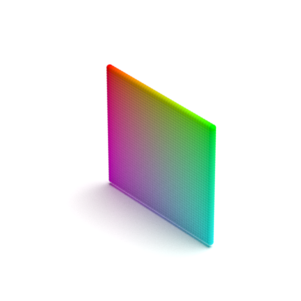
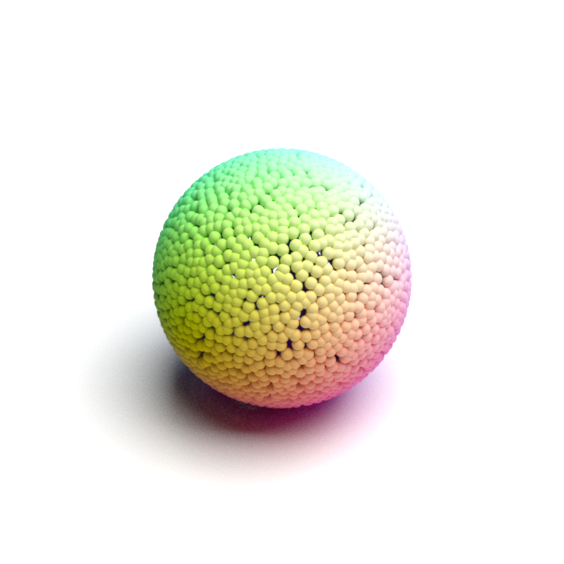
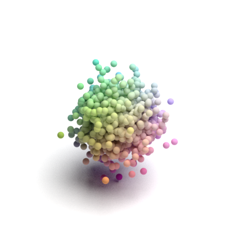
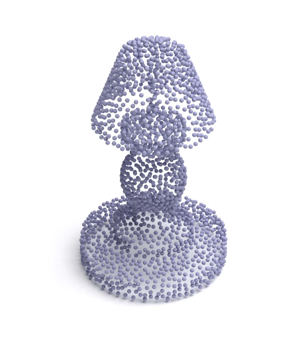
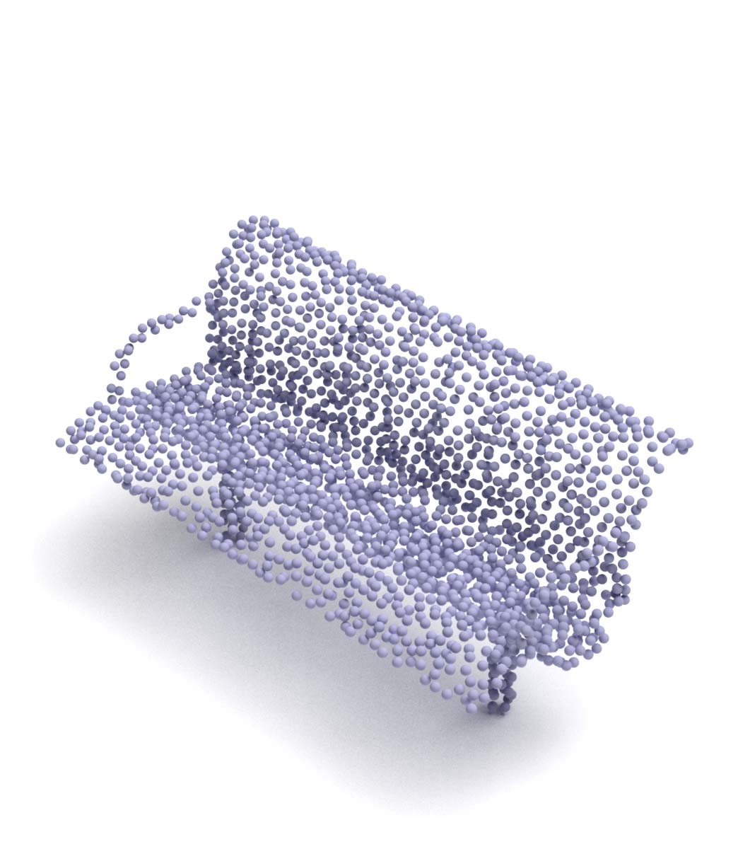
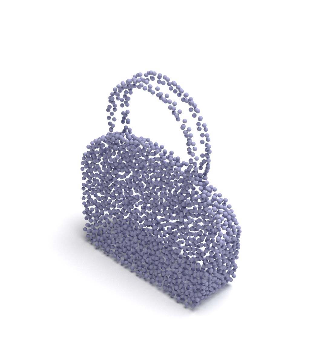
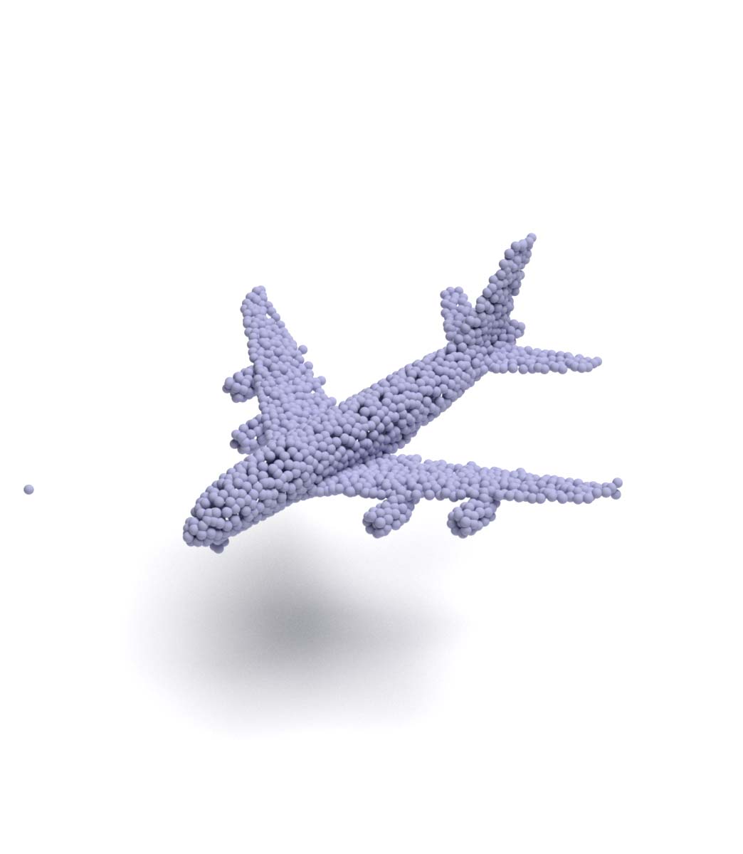
2D Plane Spherical surface Gaussian distribution
ShapeNetCore.v2 dataset
Original DGCNN_Cls (K20) DGCNN_Seg (K20)
Input Plane Sphere Gaussian Plane Sphere Gaussian Plane Sphere Gaussian
ModelNet40 dataset
Original DGCNN_Cls (K20) DGCNN_Seg (K20)
Input Plane Sphere Gaussian Plane Sphere Gaussian Plane Sphere Gaussian
CD (Chamfer Distance) scores for trained model
We provide the avg CD scores in each dataset after training, which serves as the measurement of folding performance. CD scores are multiplied by 10^4.
Results with different settings
| Encoder | K | Shape | ShapeNetCore.v2 | ModelNet40 |
|---|---|---|---|---|
| Original | 16 | Plane | 11.11 | 9.88 |
| Original | 16 | Sphere | 10.58 | 9.69 |
| Original | 16 | Gaussian | 9.63 | 11.09 |
| DGCNN_cls | 20 | Plane | 11.08 | 12.68 |
| DGCNN_cls | 20 | Sphere | 11.07 | 12.68 |
| DGCNN_cls | 20 | Gaussian | 11.18 | 12.77 |
| DGCNN_cls | 40 | Plane | 11.74 | 13.36 |
| DGCNN_cls | 40 | Sphere | 11.17 | 12.58 |
| DGCNN_cls | 40 | Gaussian | 14.77 | 17.03 |
| DGCNN_seg | 20 | Plane | 11.28 | 12.55 |
| DGCNN_seg | 20 | Sphere | 10.88 | 12.49 |
| DGCNN_seg | 20 | Gaussian | 13.36 | 15.19 |
| DGCNN_seg | 40 | Plane | 11.19 | 12.69 |
| DGCNN_seg | 40 | Sphere | 10.68 | 12.69 |
| DGCNN_seg | 40 | Gaussian | 11.95 | 13.74 |
Compare to other reconstruction methods
Models are all trained and evaluated in ShapeNetCore dataset.
| Model | Reference | ShapeNetCore.v2 |
|---|---|---|
| Latent-GAN | ICML 2018 | 7.12 |
| AtlasNet | CVPR 2018 | 5.13 |
| PointFlow | ICCV 2019 | 7.54 |
| FoldingNet (Gaussian) | - | 9.63 |
Performance analysis
Effectiveness of our reimplementation
The performance on ModelNet40 dataset is enough to validate the effectiveness of our reimplementation.
Points from sphere surface
The results of sphere show that the so-called "FoldingNet" does not restrict with folding operation. The essensce of FoldingNet decoder, i.e. MLP, is to map points from original space into new space, no matter the structure of points in original space is 2D plane grid or something else. Also, this mapping does not change neighbouring relations of points, which means adjacent points in original space are also adjacent in new space. Because point clouds are sampled from surface of an object, i.e. closed surface, the closed surface can be seen as mapped from surface of sphere just like pinching a blowing glass or Chinese sugar-figure. Thus it is reasonable to map uniformly sampled points from sphere surface to target point clouds through MLP, and as a matter of course we would consider reconstruction results for source points from sphere surface is better than 2D plane grid.
Points from gaussian distribution
Because each point is sampled independently from same gaussian distribution N(0, I), i.e. i.i.d., there is no relationship among points and the values of three axises. The reconstruction model has to learn the relationship with no prior knowledge, just like drawing on a white paper. If designed properly source points from gaussian distribution can do perfect job for reconstruction, but they can not help to extract good features for classification. This is because in order to learn the relationship the model need to focus to every details, and that is the reason why the learned model lose the ablity to extract feature in a more abstract sight, which is crucial for classification. The experimental results validate that in order to extract features suitable for classification, it is better to have some proper prior knowledge for souce points in order.
Classification v.s. reconstruction
This experiment shows that training without labels can also obtain comparable results and thus validates the effectiveness of reconstruction.
Reconstruction performance
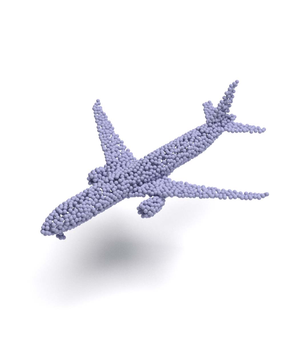
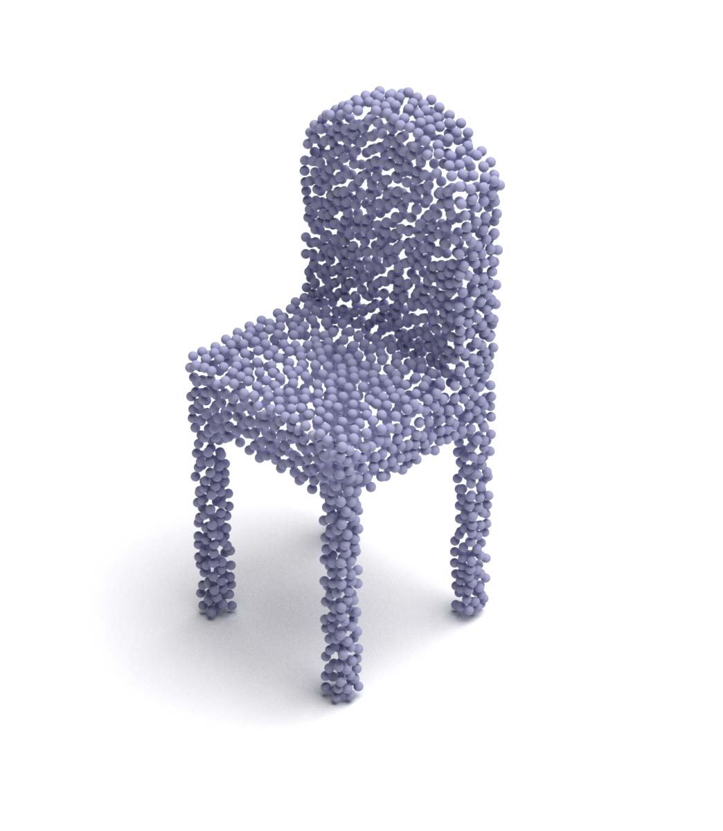
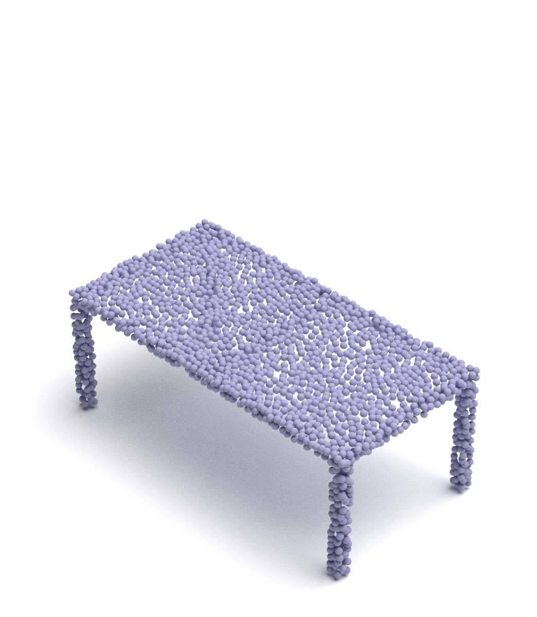
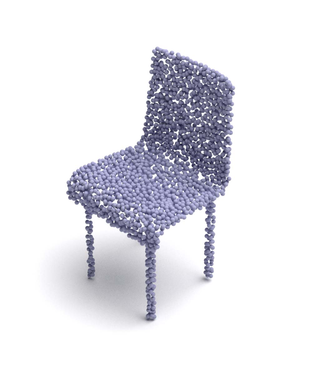
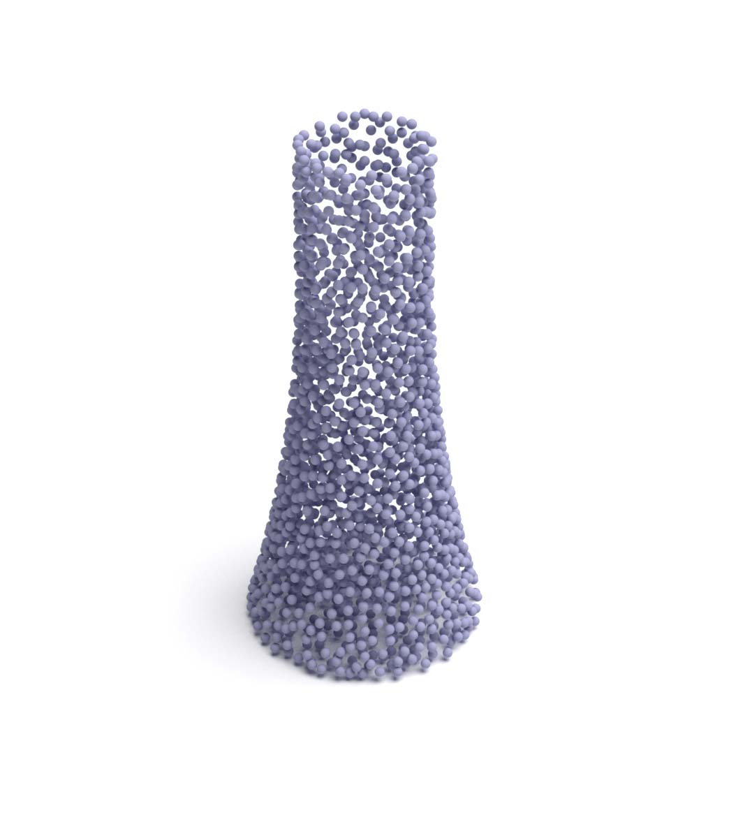
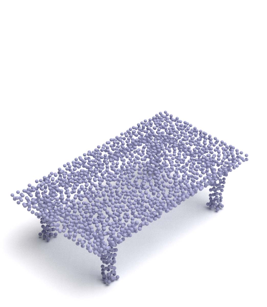
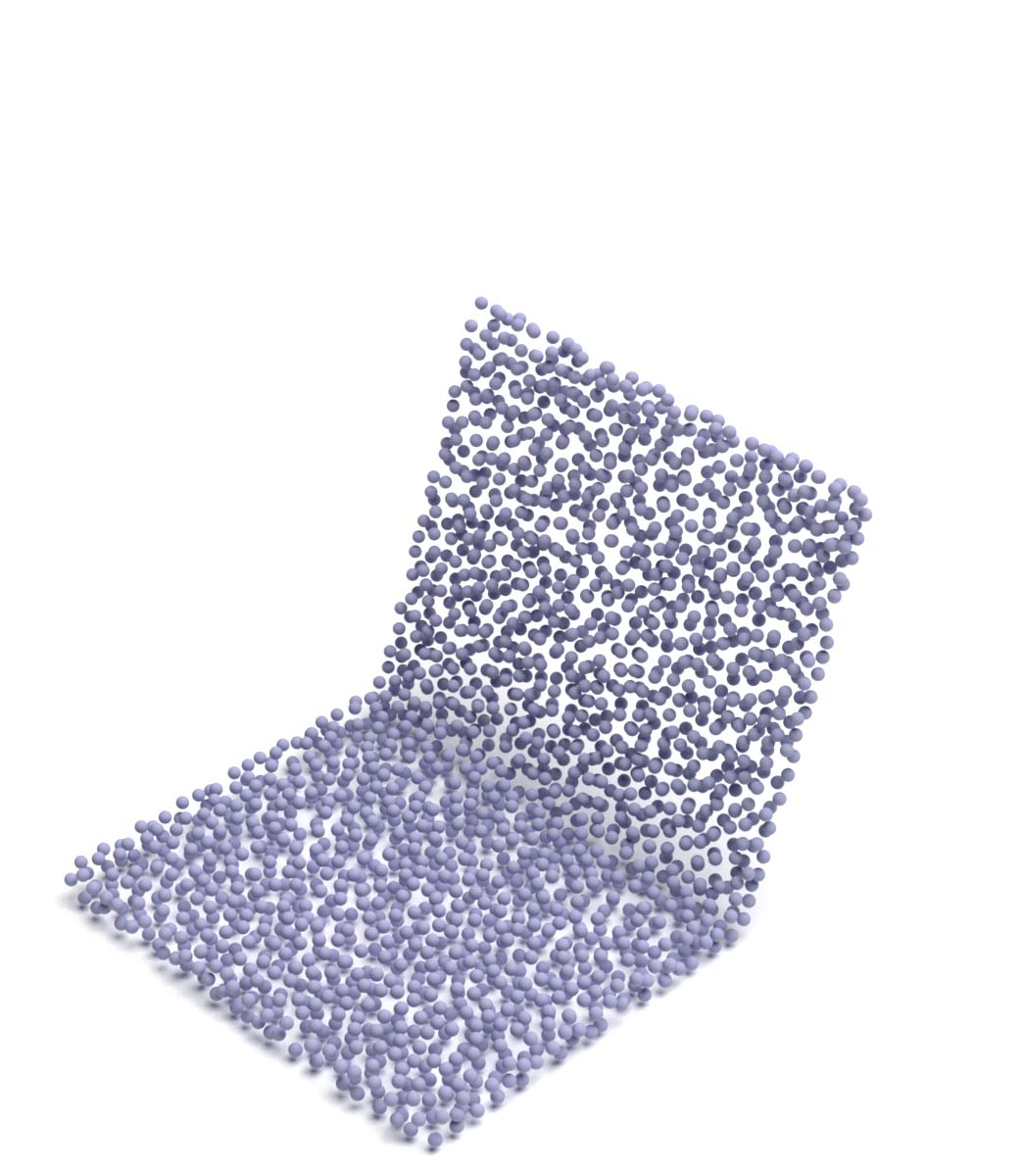
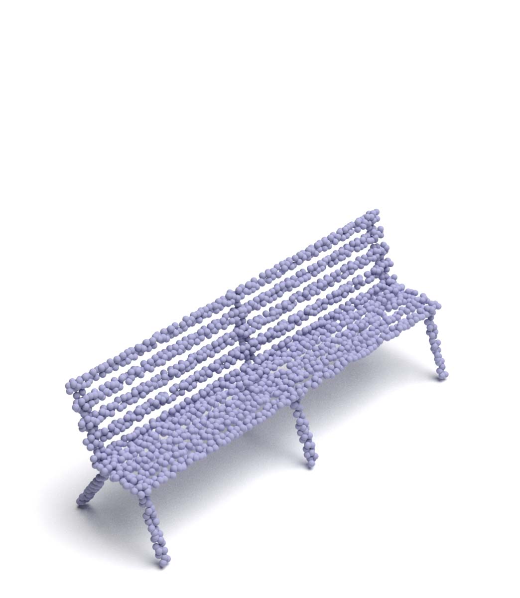
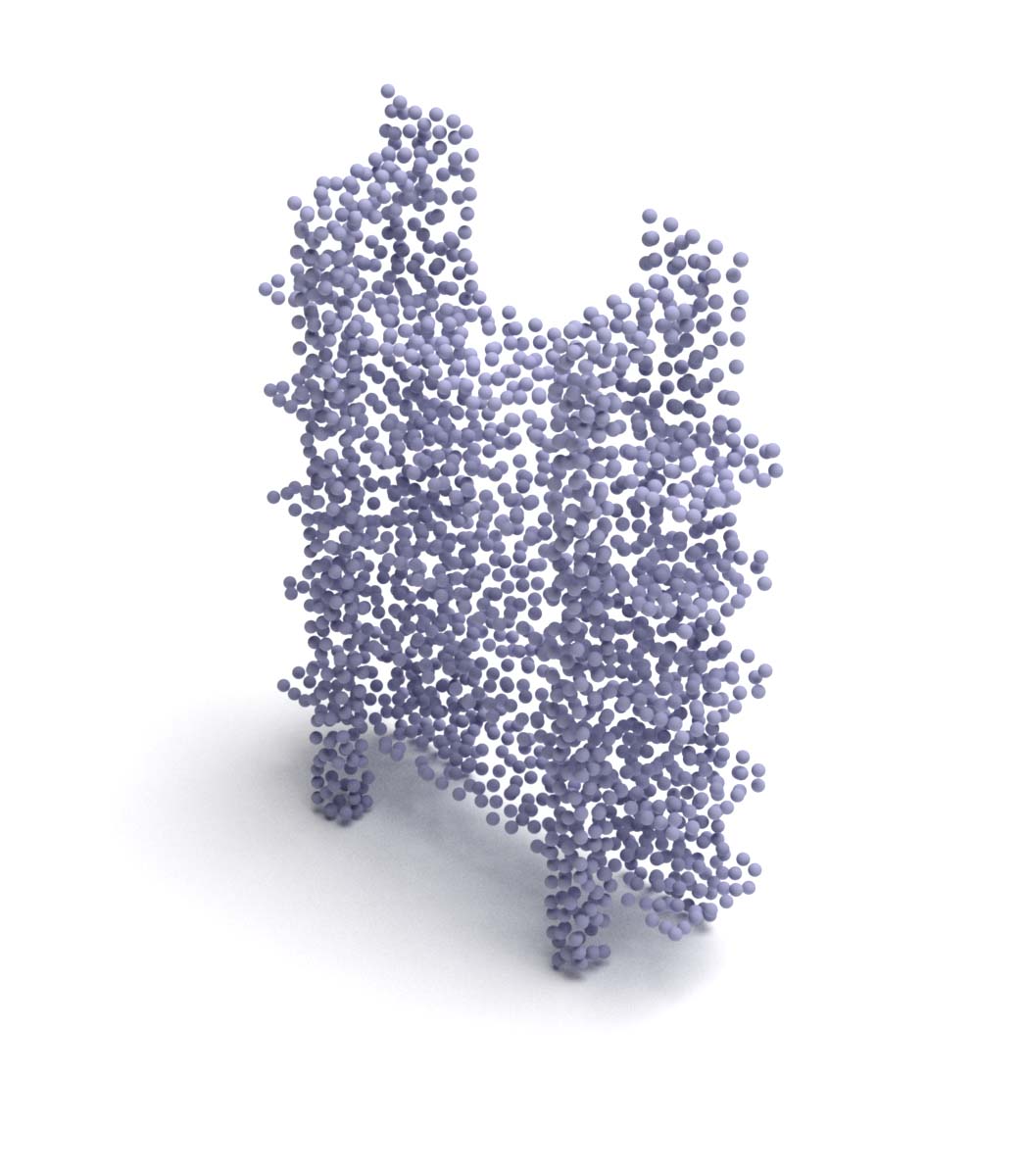
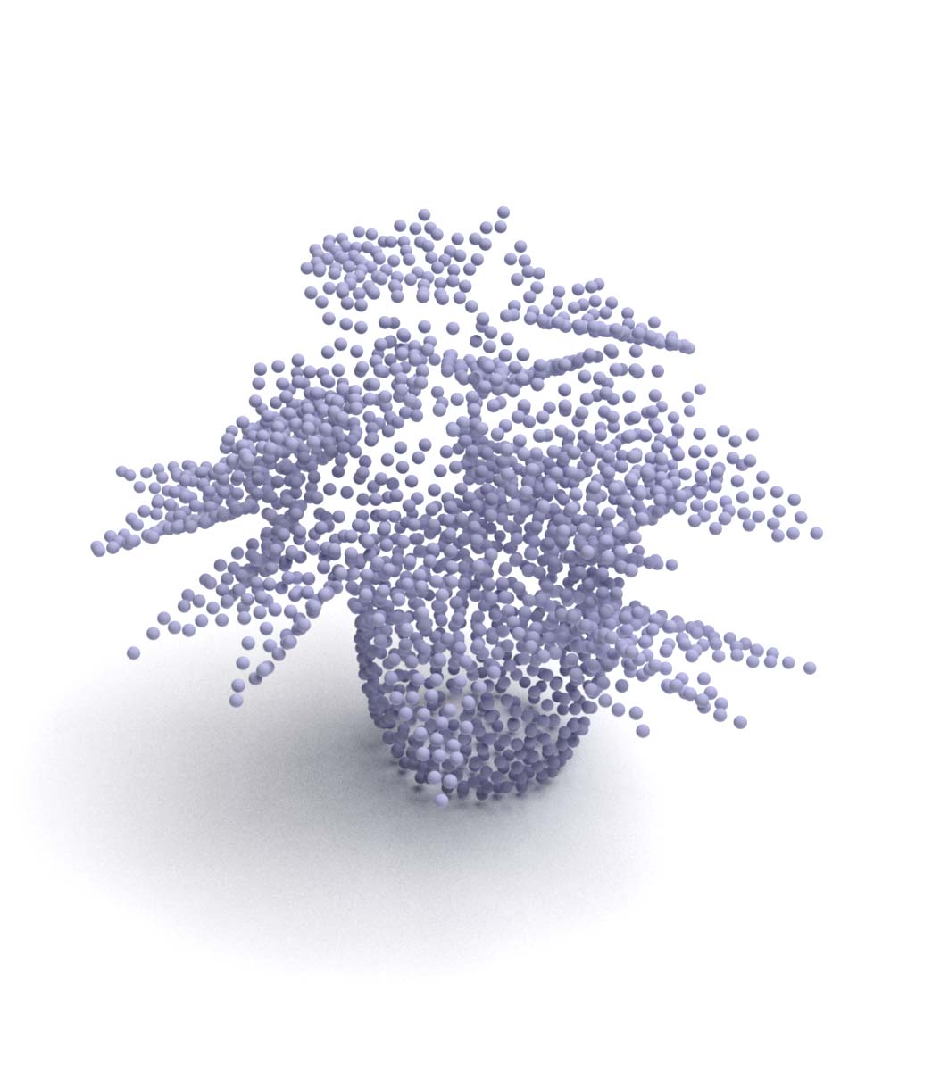
All networks run well in low curvature smooth surface, but fail in not differentiable area (crossing of planes) and high curvature surface. Because a large number of training samples have four legs, e.g. chair and table, reconstruction network also runs well in these four legs shapes. The visualized results also show characteristics of reconstructed point cloud with different corresponding source points types and encoder types.
From both visualized results and avg CD sorces, the overall reconstruction performance of ShapeNetCore.v2 dataset (training dataset) is better than ModelNet40 dataset (transfer dataset).

