

This project uses computer vision to label the lanes in a driving video, calculate the curvature of the lane, and estimate the distance of the vehicle from the center of the lane.
Steps
- Compute the camera calibration matrix and distortion coefficients given a set of chessboard images.
- Apply the distortion correction to the raw image.
- Use color transforms, gradients, etc., to create a thresholded binary image.
- Apply a perspective transform to rectify binary image ("birds-eye view").
- Detect lane pixels and fit to find lane boundary.
- Determine curvature of the lane and vehicle position with respect to center.
- Warp the detected lane boundaries back onto the original image.
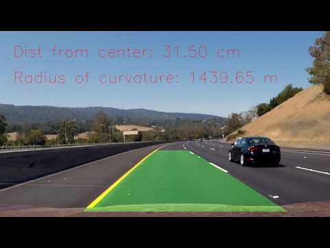
- Output visual display of the lane boundaries and numerical estimation of lane curvature and vehicle position.
git clone git@github.com:ckirksey3/lane-detection-with-opencv.git
cd lane-detection-with-opencv
If you don't already have tools like Jupyter and OpenCV installed, follow the Udacity instructions to configure an anaconda environment that will give you these tools.
jupyter notebook
To see the code in practice, execute each cell in succession by pressing shift + enter. You can also run the whole notebook in a single step by clicking on the menu Cell -> Run All.

The first step is to calibrate our camera. This is done to remove the distortion that lenses create and ensure that our lane finding algorithm could be generalized to different cameras.
We do this back by taking an image that our camera took of a chessboard and leveraging the cv2 findChessBoardCorners and calibrateCamera functions to get a camera matrix and distant coefficients. These can be used to undistort all future images from this camera.
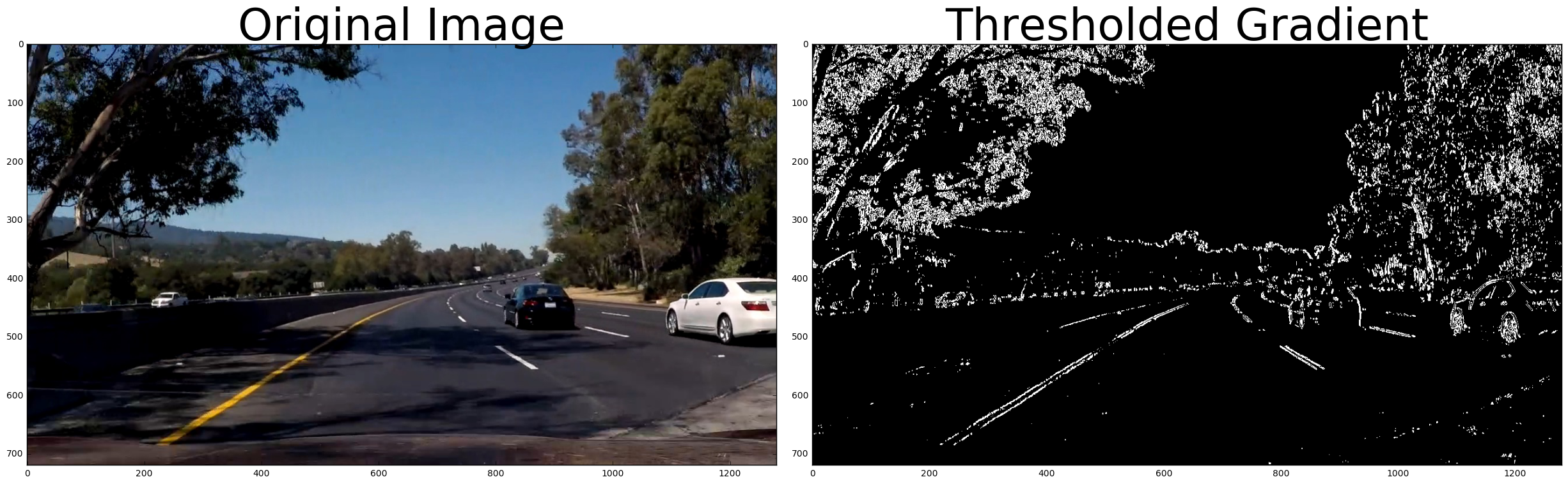
Our first iteration of computing a thresholded gradient of the road image is to apply the Sobel operator in the x direction to a greyscaled version of our image and finally compute the absolute value of the result. This isolates the gradients in the image and gives an image that we can use to isolate the lane lines. Relying on absolute value has some limitations though. As you can see from the sample image, there is still a lot of noise within the lane.

Next we try taking the maginute of the Sobel operator in both the x and y direction. By not relying too much on either directions, we're able to clear out much of the noise from the previous image.
However, there are still some thick lines in the middle that could confuse our lane detector. You can also notice that both gradients fail to detect the yellow lane at all. We'll need to fix this if we want to be able to drive anywhere with yellow lanes (aka all most everywhere).

In order to detect those yellow lanes, we can compute the direction of the gradient as the arctangent of the gradient in the y direction divided by the gradient in the x direction. This is a much noisier gradient than our magnitude gradient, but it accurately captures the identical direction of the pixels from the yellow lane.
We have some tricks for removing the rest of the noise.

Now that we've isolated the white lanes with magnitude thresholding and the yellow lanes with direction thresholding, we can combine those images with base x/y sobel thresholds to get a result that captures both lanes.
Despite lengthy tweaking of the sobel kernel size and the thresholds for the various functions, I've been unable to remove the noise in the middle of the lane. Since the markings on this section of the road are a different color than the lanes, we should be able to remove them with another technique.
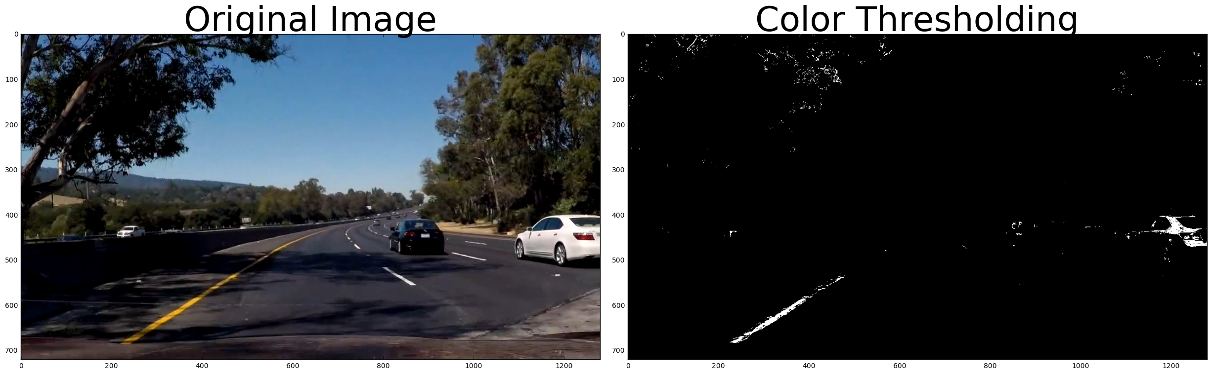
In this step, we isolat the lightness and saturation channels of the color image and then take an absolute Sobel in the x direction of the lightness channel. Finally we compute a binary that activates a pixel if it's saturated pixel is within the hardcoded threshold OR if it's scaled Sobel pixel of the lightness channel is within a separate hardcoded threshold.
After extensive trial and error with these thresholds, I was able to get ranges that effectively isolate the lanes in a variety of images.


Next, I use this bounding box to compute a perspective transformed (or "bird's eye view") version of the road image. This was one of the more challenging aspects of the project. I wanted to get a more accurate transform than I currently have, but I realized that my lane detection could still be accurate with an imperfect transform.
While working on this aspect of the pipeline, I found it helpful to compute the transform on a collection of sample images. The transform works pretty well on straight roads, but fails to transform curvy road segments accurately.
Given more time, I would use other computer vision techniques to compute the bounding box dynamically. For instance, I could use Hough lines to get a rough estimate of the lane location and horizon for computing a bounding box that adjusts for different images.

The bulk of the project is this step of taking a top-down image with the lane lines isolated and computing polynomials that fit to the left and right lane lines.
These are the steps that I take to do this:
- Divide image in half vertically and use the bottom quarter of each image to find the x coordinate with the most white pixels in it. These coordinates will be used as the estimate for the left and right lanes' starting position.
- Iterate through vertical segments of the image (starting from the bottom and moving up), detecting the most activated x-coordinate in each segment and appending to lists for the left and right lanes. Also, keep track of the y-position for each of these vertical segments.
- Leverage the lists of x and y positions for the two lanes and the numpy polyfit function to get a second-order polynomial that fits the points we detected.
- Use these polynomials to compute the radius of curvature.
- This process is fairly reliable and inaccuracies in the starting position or shape of the polynomial can generally be traced to inaccurate input images.
Once we've computed the fit polynomial for the left and right lanes, we can use it in conjuction with y values from the vertical segments that we iterated through to plot a fill space on the image, highlighting the lane.
This project was able to make steady, gradual process by breaking each step of the pipeline into a separate function and slowly iterating on each one.
One of the key opportunities for improvement would be to apply a minimum threshold for lane detection when building my polynomial. For instance, if I'm processing an image where the left lane has very little white pixels at all, I'd automatically calculate that and just reuse the lane polynomial from the previous frame.
There are still some limitations on the gradient itself. Occasionally it will detect creases in the road (left from construction) as lane lines. I could probably reduce the impact of this be enforcing a certain lane width and rejecting any lane estimates that fall outside of that width.
This was a very interesting project and I enjoyed learning the nuances of the producing the lane polynomial. The end product was pretty satisfying too as it looks much smoother than the original project with rough lane estimates.