chaudharyachint08 / Stock-Analyzer

Using Technical, Fundamental, and Sentimental Analysis with Machine Learning

Stock Analyzer

Applying technical, fundamental, and sentimental stock analysis with Machine Learning Models

Table of Contents

• Project Purpose
• Project Overview
• Data Sources
• Data Gathering and Cleaning
• Exploring Data
• Classification
• Time Series
• Sentimental
• Frontend and Presentation
• Next Steps

Project Purpose

Three of the most popular stock analysis methods are technical, fundamental, and sentimental analysis. Perhaps Machine Learning can be used to remove the human element from these methods of analysis. For fundamental analysis, classification models were used to determine if a stock would be a Buy, Sell, or Hold. For technical analysis, time series models were used to forecast the general direction of the stock price. For sentiment analysis, NLP tools were used such as NLTK's VADER to determine the public's opinion and feeling towards a stock. The hope would be that these machine learning models would enhance and improve the current methods of analysis.

Project Overview

1. Collected data from three different web sources by using webscraping or API calls.
   • Yahoo Finance for Time Series data
   • Stockpup for Fundamental data
   • Twitter for sentimental data
2. Data cleaning and Exploratory Data Analysis
   • Fundamental data was cleaned and formatted into a Pandas DataFrame.
   • Time series data was downloaded as daily data then resampled into weekly and monthly intervals.
   • Sentimental data was formatted into a Pandas DataFrame.
3. Modeling
   • Fundamental data was then used to train several different classification models.
   • Time series data was fitted and trained to two time series models.
   • Sentimental data did not require any modeling.
4. Presentation and Frontend
   • Streamlit was used to create a frontend for each form of analysis with their respective machine learning models.
5. Next Steps

Data Sources

Data sources for each different method of stock analysis required different websources:

• Stockpup.com contained 765 stock tickers and quarterly reports for each. This was webscraped using BeautifulSoup and stored as separate DataFrames in a dictionary then pickled for later use.

• Yahoo Finance contained the daily prices for each stock searched and could be downloaded individually as a CSV file. Selenium was used to automate the downloading process for any stock entered.

• Twitter was used to source 200 tweets about any stock desired. Twint was used to simplify the tweet webscraping process instead of Twitter's API due to the API's limited nature.

Data Gathering and Cleaning

• BeautifulSoup was used to scrape Stockpup.com: Retrieving Data

• Selenium was used to scrape Yahoo Finance: Price Scraping

• Twint was used to scrape Twitter: Twitter Scraping

Data Cleaning:

Fundamental Data from Stockpup.com

Fundamental Data Cleaning

Every Quarterly Report was downloaded as a Pandas DataFrame and stored in a dictionary of DataFrames.

For each DataFrame:

1. Index was set as datetime from the "Quarter end" column.

2. 'None' values were replaced with 0 and converted to numerical values.

3. Replaced current values with the differences between each Quarter with respect to each Stock. (Also replaced infinite values with 1 and -1. Also any new NaNs were replaced once again with 0.

4. Created new columns showing the future Quarter's price high/low % change then created classes based on those values. - If the future price high and future price low increased by 5% or more, then the present Quarterly report is classified as a Buy. - If the future price low and future price high decreased by 5% or more, the the present Quarter report is classified as a Sell. - Otherwise, the present Quarterly report is classified as a Hold.

5. First and Last rows were excluded because the last row has no data to calculate the difference with and the first row has no data showing the future price high and low.

6. All Quarterly Reports were then combined into one DataFrame.

7. Checked for any remaining NaNs. Columns with less than 500 unique values were excluded because their impact would be small if nothing at all.

8. Resetted Index

9. Classes were balanced by removing excess rows to match the class with least amount of rows.

10. Finally, the final DataFrame was exported as a pickle file for modeling.

Sentimental Data from Twitter

Sentimental Data Cleaning

Twint, a module used for scraping tweets, was used over the Twitter API because of Twint's flexibility and freedom.

• 200 Tweets were scraped for the sake of brevity in the presentation. More tweets can be scraped if desired.
• Twint searched for any stock given based on the cashtag($) (e.g. $AMD).
• Retweets were filtered out.
• No media such as pictures or video.
• English tweets only.
• No tweets referring to web links.
• All tweets were then stored into a Pandas DataFrame.

Technical Data from Yahoo Finance

Technical Data Cleaning

Not much cleaning was required for the technical data

• Each stock had their price data read into a Pandas DataFrame
• Index was set as a Datetime index from the 'Date' column
• Values were converted to numerical values.
• All columns were excluded except for closing price.
• Data was then resampled into weekly and monthly formats but still retaining daily as well.
• Last 1000 periods of data was used because they represent the current market climate better than older data.
• Finally, each DF of resample data was exported into a pickle file.

Exploring Data

Fundamental Exploration

Visualization of the Class Balance between Buys, Holds, Sells.

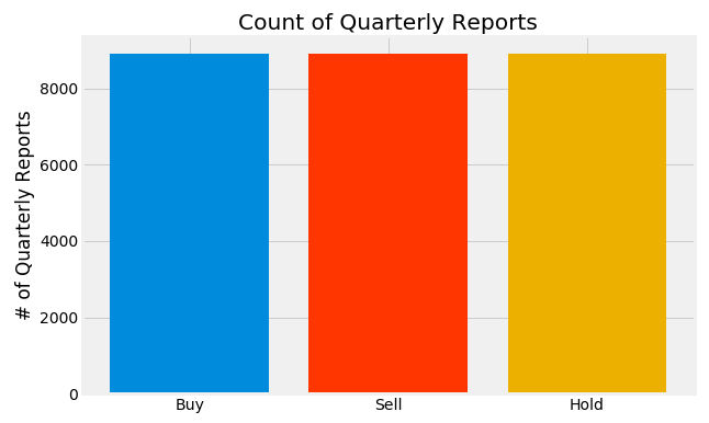
Classes were balanced during the cleaning process. This is done so that randomly guessing a class label will result in a 33% success rate.

Visualization of the correlations between each feature and the target variable (Decision).

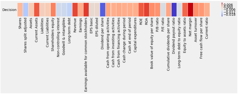
Here the most influential features to the 'Decision' can been seen.

Visualization of the important features.

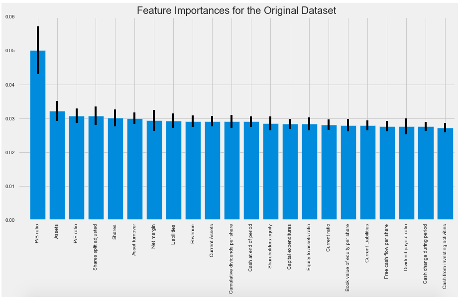
Using the ExtraTreesClassifier, the most important features were ranked and plotted. According to the simple classifier, "P/B Ratio" turned out to be the most important feature when it comes to determining the correct class label.

With the most important features ranked and sorted, the unimportant features were removed from the dataset and the top 10 were kept (along with the top 5 and top 20 features for comparison's sake).

Technical Exploration

For exploration of the technical/time series data, the last 1000 periods were used instead of the entire dataset because those 1000 periods better represent the current market climate. These 1000 periods were derived from the Daily data as well as the Weekly and Monthly. Weekly and Monthly were resampled Daily Data.

Visualization of the Daily Differences in Price data

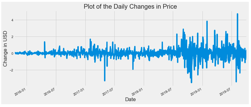
Differencing the data was done to check for sationarity. This step is necessary for any ARMA modeling.

Visualization of the ACF and PACF

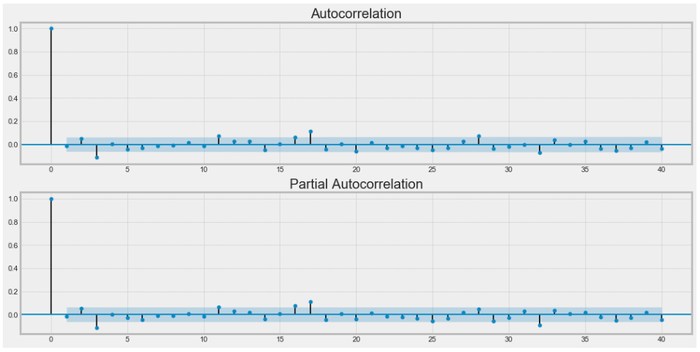
The ACF and PACF was done to check for any seasonality with the time series data.

Sentiment Exploration

Exploration of the Sentiment data was done as the final presentation of sentiment analysis because no modeling was done to the data. A more in-depth look into the sentiment data is under the Sentimental section of this README.

Classification

For the fundamental data, classification models were used to determine if a stock was a Buy, Hold, or Sell. Numerous Classification models were implemented to find the best performing model. These models are:

- XGBoost
- AdaBoost
- Random Forest
- SVM
- KNN
- Neural Network

Out of all these Classification models, XGBoost performed the best:

- Training Score: 47%
- Testing Score: 45%

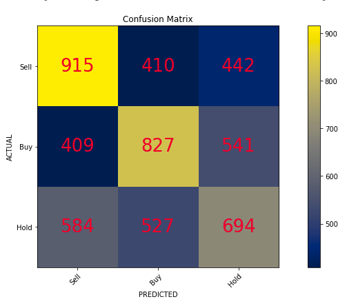
XGBoost's confusion matrix

This confusion matrix was created from XGBoost modeling the top 10 features from the original dataset.

Most of the other models were performing with scores around 35% - 43% range for both their Testing and Training set.

Feature Selection and Feature Engineering for Classification Features

Feature Selection and Engineering

Many different approaches to the fundamental features were considered to improve the performance of the models.

These approaches were:

• Feature Interactions
• Principle Component Analysis (PCA)
• Feature Importance
• Scaling the Data

Feature Interactions

Through the use of SKlearn's PolynomialFeatures and StandardScaler, the features from the original dataset all interacted with each other. Any feature that involved Price was removed to prevent any data leakage as well as the class labels and self-interacting features. After removing those features, a little over 700 features still remain.

Principle Component Analysis (PCA)

Because there are a little over 700 features now in the dataset, many features must be removed to simplify the computing process as well as to avoid the "Curse of Dimensionality". To lessen the amount of features, PCA was utilized, which was able to reduce the number of features from 700+ to 79.

(E.g. PCA Modeling)

After using many different models on the data from the reduced number of features, the training and testing scores did not perform significantly better than the model scores on the non-interacted features.

Feature Importance

By using the top 20, top 10, and top 5 most important features derived from the ExtraTreesClassifier, different modeling scores were captured from various models. This was done to compare the performance of each model under the different number of top features.

(E.g. Top 20 feature modeling)

After modeling each number of important features, the top 10 most important features proved to be the best performing set of features to model.

Scaling the Data

Scaling the data using SKlearn's StandardScaler improved model performance over unscaled data.

Scaled Modeling vs. Unscaled Modeling

Deep Learning Neural Network for Classification

Neural Network Classification

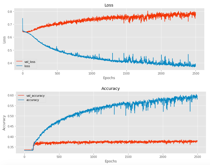
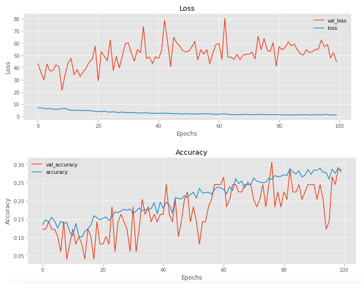
To fully explore the classification aspect of the problem, a neural network was attempted with the top 10 features. A variety of layers, epochs, and nodes were experimented with to find the optimum amount.

After training the neural network for many hours and seeing no significant improvements over the machine learning models, it was concluded that a neural network for this problem was not the best solution. Many of the other machine learning classification models performed better than the best scored neural network.

Time Series

For the Technical data/analysis, Time-series models were used to forecast the next set of stock prices for any stock.

Numerous time-series models were utilized to find the model with the best performance. These models were:

• SARIMAX
• FaceBook Prophet
• Recurrent Neural Network

Each model only had one input: Price. The logic behind only using price was to observe if a model would be able to pick up on any price patterns to predict on. Prediction based on price patterns is the basis of technical analysis.

SARIMAX Modeling

SARIMAX Model

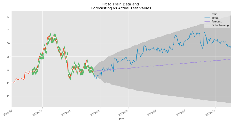
SARIMAX was the first model used to forecast and analyze a stock. The train and test sets were split in order so that the test set contained the most recent values which was 20% of the original dataset.

• SARIMAX had to be GridSearched to find the optimum parameters. This was done using a custom function that would loop through each possible combination of values for SARIMAX using the entire dataset.
• Once optimal parameters were found, they were used to fit the model to the training set and then the forecasted values and the actual values (test values) were visualized.
• Finally, the entire dataset was fitted with the optimal parameters and then the forecasted values and confidence intervals were forecasted.

FaceBook Prophet Modeling

Facebook Prophet Model

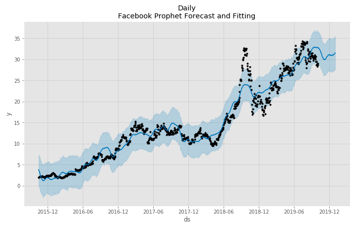
Facebook Prophet was the next model used to forecast a stock's future prices. Train, test, split was not done here and searching for optimal parameters was not required.

• At the core of FBProphet is an additive regression model.
• FB Prophet is able to produce high quality forecasts with much less effort and in less time than other Time Series models.
• In order to create forecasted prices, FBProphet needs to predict from a newly created dataframe of future dates.
• These predictions and forecasts are presented as seen above.
• Facebook Prophet also allows a visualization of the components of the forecast.

Recurrent Neural Network (LSTM)

RNN LSTM Model

A recurrent neural network (specifically a Long Short Term Memory Network) was attempted to see if its predictions were better than normal time series models.

• An LSTM was used specifically because it is best suited for time series data.
• Many layers, nodes, and epochs were experimented with to find the best performing network.
• Data had to be split into sequences; a function was written for this exact purpose.
• Each sequence has a number of periods to look back and a number of periods to predict.

After training the neural network for several hours, the predictions were reasonably realistic but time to train was extremely time consuming and only stock was able to be forecasted/predicted.

Being able to use a neural network flexibly and quickly is not possible with the current resources. As a result, the Facebook Prophet model was determined to be the best option for stock time series data.

Sentimental

Sentiment Analysis

Sentimental Data was collected from Twitter, which was made possible by using the module Twint. Twint was used over Twitter's API because Twint is more flexible and less limited than the Twitter API.

• 200 tweets were gathered for any stock requested by using its cashtag($). (More tweets could be gathered but for the sake of time and efficiency, 200 was the limit for now).
• NLTK's VADER was used to find the sentiment score for each tweet, which ranged from -1 to 1.
• This score was then assigned to a new column for the tweets.
• Each score was then classified as positive, negative, or neutral using a custom function.
• The new dataframe contains only the tweet, sentiment (-1 to 1), and feeling (pos, neg, neu).
• Visualization of the data was the next step after the data was formatted correctly.
• No modeling was required for this entire process.

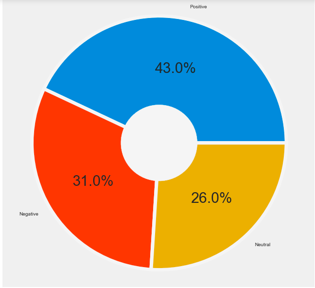
A donut chart was used to visualize the count of tweets (displaying the percentage of the 200 tweets)

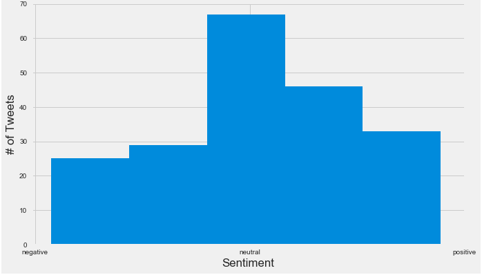
A histogram distribution was used to visualize the sentiment score of the tweets with x-ticks of -1, 0, and 1 replaced with negative, neutral, and positive respectively.

By observing these sentiment visualizations, the hope is that a user would be able to determine the general opinion of the stock without having to look through various tweets themselves.

Frontend and Presentation

Final presentation Streamlit frontend

In order to present the Technical, Fundamental, and Sentimental analyses in a visually appealing format, Streamlit was implemented as a frontend.

Before an actual frontend with Streamlit was considered, a normal Jupyter Notebook was used to present the visualizations of every analysis: Presentation without Streamlit

Once an outline of the presentation in a jupyter notebook was established, then a presentation utilizing Streamlit was able to be used by opening the python file using streamlit's command.

The frontend app or presentation is interactive allowing the user to select any stock from a given list (765 stocks from Stockpup) to analyze. Once a stock is selected, the user will be able to choose which form of analysis (fundamental, technical, and sentimental) to use on the selected stock.

• If the user selects Fundamental, then a classification model (XGBoost) is ran on the newest Quarterly Report data. The classification probability is then visualized and presented to the user.

• If the user selects Technical, then the user determines how long into the future they want to forecast by using a slider from 0 to 365 days. Next, Selenium is used to scrape the latest closing prices from Yahoo Finance, which is then modeled using Facebook Prophet. FBprophet then visualizes the forecast and displays it to the user.

• If the user selects Sentimental, then Twint gathers the latest tweets regarding the selected stock. NLTK's VADER then analyzes the sentiment which is later visualized with the donut chart and histogram chart.

Alternatively, a user is able to select all three methods of analysis.

Next Steps

• To truly gather the most up to date quarterly reports for the classification model, webscraping other websites besides Stockpup must be done.
• Time Series models could possibly use other exogenous variables from Technical indicators such as MACD, Stochastic, RSI, etc.
• More time for neural network training to find the optimum number of layers/nodes by gridsearching the hyperparameters with potentially the TPOTClassifier or other methods.
• Possibly a closer examination of the sentimental data from Twitter. Also, maybe scrape from Stocktwits for more relevant sentimental data.