brownag / grundo

Digital Soil Mapping (DSM) From The Ground Up!

{grundo}

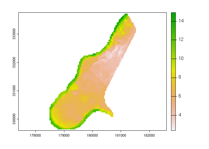
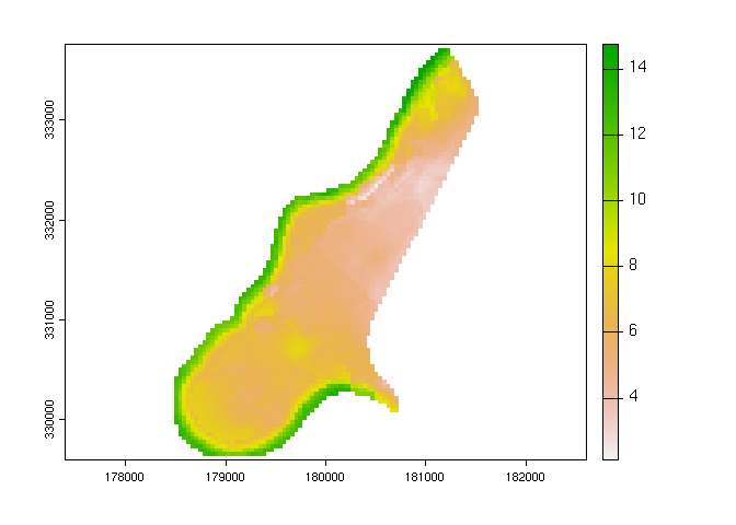
Welcome to the “{grundo} mundo.” The goal of {grundo} is to provide a simple, modern R interface for creating gridded maps of soils, with a focus on preparing observational data for statistical analysis and evaluating the models that predict soil properties or classes.

The package also seeks to provide a light compatibility layer between the {terra} and {gstat} packages. Note you do not need to use {terra} classes, {sf}, {sp}, and {stars} are fully supported.

{grundo} Models

A {grundo} model includes a primary model trained to predict variable using values extracted from predictors at samples locations. This model is selected with the model argument from one of several options described in subsequent sections.

Each run of grundo::grundo() includes an ordinary kriging step to interpolate residuals from the primary model and estimate the spatial pattern of the errors in the training area.

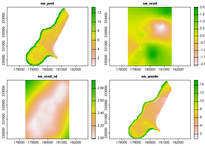
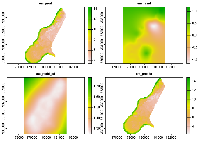
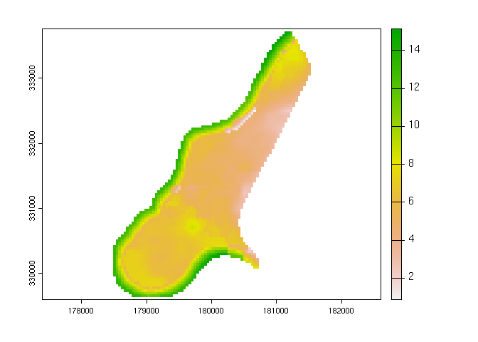
The first layer of resulting prediction SpatRaster is the primary model prediction. The second layer is the interpolated residuals, and generally will have positive and negative values distributed around zero. The sum of the two grids will give a more realistic estimate of values in the training area given the known, observed point values.

• If there is no significant spatial component to the errors, the residual kriging value is the mean value of the residual errors from the training data. This mean error value is also assumed for predictions made outside the extent of the training data.

Installation

You can install the development version of {grundo} from GitHub with {remotes}:

if (!require("remotes")) install.packages("remotes")
remotes::install_github("brownag/grundo")

Example

This example uses the classic meuse dataset to demonstrate prediction of surface soil organic matter content (%) along the Meuse River. These datasets have been augmented with additional DEM-derived (SRTM) data for more continuous numeric predictors.

library(grundo)
library(terra)
#> terra 1.6.47

samples <- vect(system.file("extdata", "meuse.gpkg", package = "grundo"))
predictors <- rast(system.file("extdata", "meuse.grid.ex.tif", package = "grundo"))

## to use classic `meuse` datasets from {sp} package
# data(meuse, package = "sp")
# data(meuse.grid, package = "sp")
# predictors <- rast(meuse.grid, crs = "EPSG:28992")
# samples <- vect(meuse, geom = c("x", "y"), crs = "EPSG:28992")

Dependent Variable

First we select a dependent variable that is a soil property, such as "om" (surface soil organic matter percentage).

variable <- "om"

Predictors and Samples

Next we will set up a {terra} SpatRaster containing the grids of our predictors, and a SpatVector of points where soil properties have been measured. For this example we construct these objects from data.frame datasets defined in the {sp} package.

# remove observations that are missing organic matter %
samples <- samples[!is.na(samples[[variable]][[1]]), ]

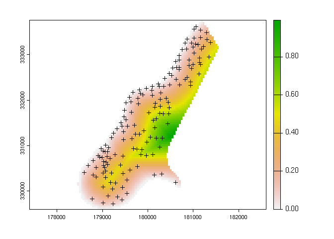
# visual inspection
plot(predictors[[3]])
points(samples, pch = "+", cex = 1)

There are several other soil properties of interest that can be used, see names(samples)

names(predictors)
#> [1] "part.a"    "part.b"    "dist"      "soil"      "ffreq"     "elevation"
#> [7] "slope"

names(samples)
#>  [1] "cadmium"   "copper"    "lead"      "zinc"      "elev"      "om"       
#>  [7] "lime"      "landuse"   "dist.m"    "ID"        "part.a"    "part.b"   
#> [13] "dist"      "soil"      "ffreq"     "elevation" "slope"

Models

Cubist model with Cubist::cubist()

grundo() supports {Cubist} models with model="cubist"

# cubist with {Cubist} + OK residuals
x <- grundo(
  predictors = predictors,
  samples = samples,
  variable = variable,
  model = "cubist",
  vgm_model = "Exp"
)
#> Loading required namespace: Cubist
#> Warning in gstat::fit.variogram(grundo::variogram(samples, rfm),
#> gstat::vgm(vgm_model)): No convergence after 200 iterations: try different
#> initial values?
#> [using ordinary kriging]
#> [using ordinary kriging]

plot(x$result)

plot(sum(x$result[[1:2]]))

Random Forest model with ranger::ranger()

grundo() supports {ranger} (Random Forest) models with model="ranger"

# random forest with {ranger} + OK residuals
y <- grundo(
  predictors = predictors,
  samples = samples,
  variable = variable,
  model = "ranger",
  vgm_model = "Exp"
)
#> Loading required namespace: ranger
#> Warning in lapply(r, as.numeric): NAs introduced by coercion

#> Warning in lapply(r, as.numeric): NAs introduced by coercion
#> Warning in gstat::fit.variogram(grundo::variogram(samples, rfm),
#> gstat::vgm(vgm_model)): No convergence after 200 iterations: try different
#> initial values?
#> [using ordinary kriging]
#> [using ordinary kriging]

plot(y$result)

plot(sum(y$result[[1:2]]))

grundo() “Ensemble”

We can take the average of several grundo() runs for an “ensemble” estimate.

plot(mean(c(sum(x$result[[1:2]]), sum(y$result[[1:2]]))))