bchao1 / Fun-with-MNIST

Playing with MNIST. Machine Learning. Generative Models.

Fun with MNIST

All MNIST images are padded to 32 * 32 for the sake of convenience. The MNIST data is already downloaded in the ./data directory.

Table of contents

• Basics

  • MNIST Classification
  • PCA: Principle Component Analysis on MNIST
  • tSNE: t-Nearest Neighbors Embedding on MNIST

• Generative Models

Model	Reference	Difference from orignal GAN
Autoencoders
Vanilla Autoencoders	https://www.cs.toronto.edu/~hinton/science.pdf	N/A
VAE: Variational Autoencoders	https://arxiv.org/abs/1312.6114	N/A
GANs
GAN: Generative Adversarial Networks	https://arxiv.org/abs/1406.2661	N/A
Adversarial Autoencoders	https://arxiv.org/abs/1511.05644	Encoder generates samples from a prior distribution.
WGAN: Wasserstein's GAN	https://arxiv.org/abs/1701.07875	No sigmoid at discriminator output, weight clipping.
WGAN-GP: Improved Wasserstein's GAN	https://arxiv.org/abs/1704.00028	Same as WGAN but replaces weight clipping with gradient penalty.
InfoGAN: Information maximizing GAN	https://arxiv.org/abs/1606.03657
ACGAN: Auxiliary Classifier GAN	https://arxiv.org/abs/1610.09585	Generator has label information, discriminator also classifies.
Conditional GAN	https://arxiv.org/abs/1411.1784	Both generator and discriminator has label information
VAE-GAN: VAE + GAN	https://arxiv.org/abs/1512.09300
BEGAN: Boundary Equilibrium GAN	https://arxiv.org/abs/1703.10717
EBGAN: Energy-based GAN	https://arxiv.org/abs/1609.03126	Models discriminator as an autoencoder
LSGAN: Least Squares GAN	https://arxiv.org/abs/1611.04076	No sigmoid at discriminator output, measures L2 distance of image scores.

• Domain Adaptation

Model	Reference
CycleGAN	https://arxiv.org/abs/1703.10593
Coupled GAN	https://arxiv.org/abs/1606.07536
UNIT	https://arxiv.org/abs/1703.00848
pix2pix	https://arxiv.org/abs/1611.07004

• Others

Topic	Reference
Semi-supervied learning with SGAN	https://arxiv.org/abs/1606.01583
Transfer Learning
Spatial Transformer Networks

Basics

MNIST Classification

Back to the basics: implemeting a CNN to classify digits. The architecture is a feature extrator(convolutional layers) + a fully connected layer that outputs class probabilities.

CONV(in:1, out:64, k4s2)->LeakyReLU(0.2)->BN(64)->
CONV(in:64, out:128, k4s2)->LeakyReLU(0.2)->BN(128)->
CONV(in:128, out:256, k4s2)->LeakyReLU(0.2)->BN(256)->
CONV(in:256, out:512, k4s2)->LeakyReLU(0.2)->BN(512)->
FCN(2048, 10)->Softmax

Results

Accuracy	Notes
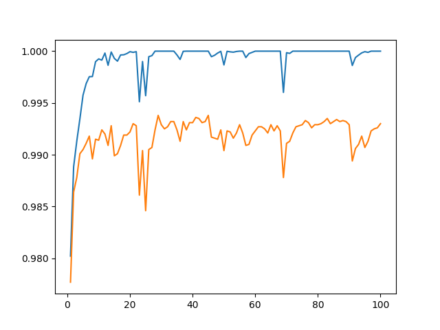	blue: train, orange: test

PCA on MNIST

PCA

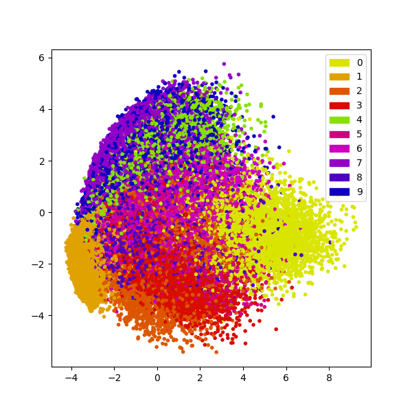tSNE on MNIST

tSNE

Generative Models

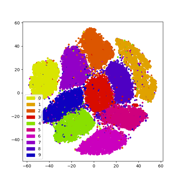In the following generative models, some of them (all GANs) are modified from the following model architecture (DCGAN-like):

• Downsampling networks(discriminator, encoders)

nn.Sequential(
                nn.Conv2d(1, 64, 4, 2, 1, bias = False),
                nn.LeakyReLU(0.2),
                nn.Conv2d(64, 128, 4, 2, 1, bias = False),
                nn.BatchNorm2d(128),
                nn.LeakyReLU(0.2),
                nn.Conv2d(128, 256, 4, 2, 1, bias = False),
                nn.BatchNorm2d(256),
                nn.LeakyReLU(0.2),
                nn.Conv2d(256, 512, 4, 2, 1, bias = False),
                nn.BatchNorm2d(512),
                nn.LeakyReLU(0.2),
                nn.Conv2d(512, self.latent_dim, 2, 1),
                nn.Sigmoid()
                )

• Upsampling networks(generator, decoder)

nn.Sequential(
                nn.ConvTranspose2d(self.latent_dim, 512, 4, 2, 1, bias = False),
                nn.BatchNorm2d(512),
                nn.ReLU(),
                nn.ConvTranspose2d(512, 256, 4, 2, 1, bias = False),
                nn.BatchNorm2d(256),
                nn.ReLU(),
                nn.ConvTranspose2d(256, 128, 4, 2, 1, bias = False),
                nn.BatchNorm2d(128),
                nn.ReLU(),
                nn.ConvTranspose2d(128, 64, 4, 2, 1, bias = False),
                nn.BatchNorm2d(64),
                nn.ReLU(),
                nn.ConvTranspose2d(64, 1, 4, 2, 1, bias = False),
                nn.Sigmoid()
                )

Some models (eg. autoencoders, vae) are just simple fully-connected layers. I did not replicate all settings in the orignal papers since it is more important to capture the overall concept.

---

---

[ Deep autoencoders ]

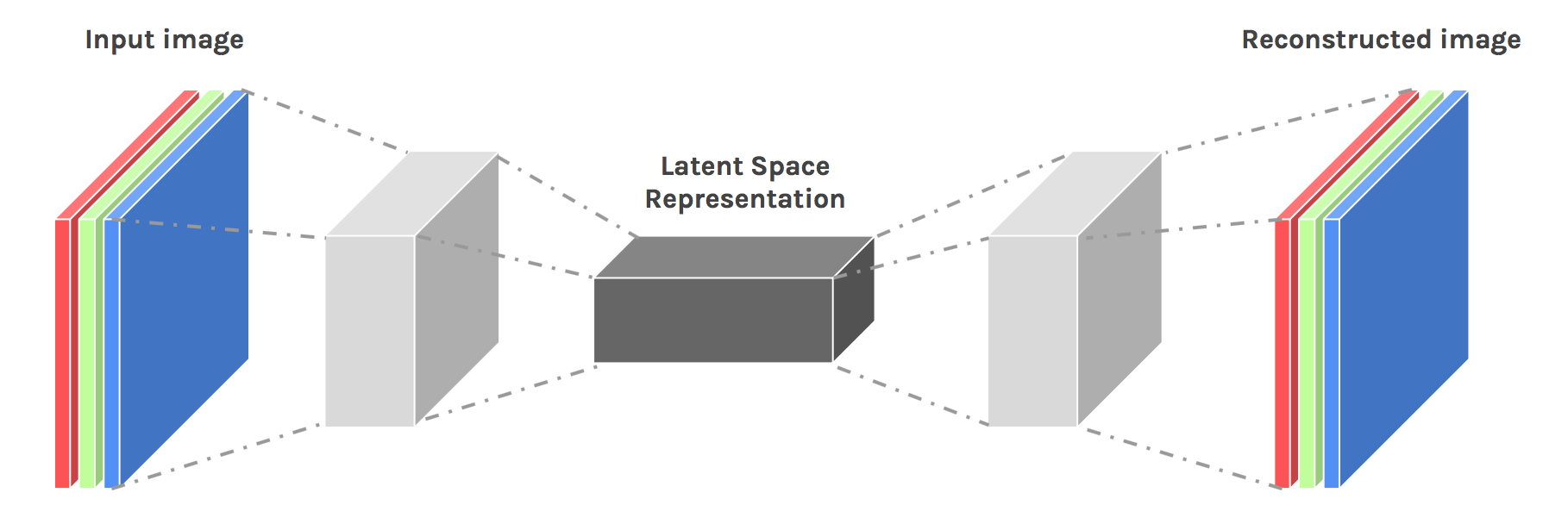
Autoencoders are relatively simple generative models compared to the state-of-the-art GANs. The basic idea is to project a high-dimensional vector (eg. an image) to a low-dimensional latent space, and then reconstruct the image based on this latent code representation.

Structure

Results

Reconstruction from 100 dimension latent code.

Original	Reconstructed

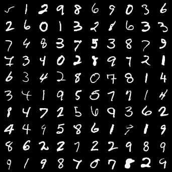After 50 epochs, images can almost be perfectly reconstructed.

---

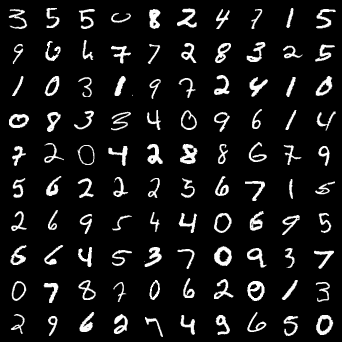
Reconstruction from 2 dimension latent code. (last layer of the encoder with sigmoid, hence the code value is clipped between 0 and 1).

Original	Reconstructed

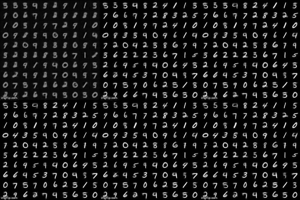The results are blurry since images are reconstructed from 2-dimensional codes, where the original images are 32 * 32 = 1024 dimensional vectors. Much information is lost after encoding process.

---

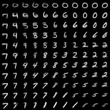
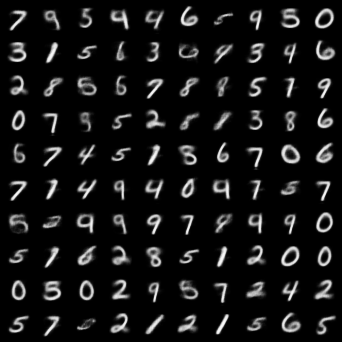
We can also generate images on the 2-dimensional manifold. From the results below, we can see that there seems to be some correlation between the digit shapes and the dimenions.

(0,1) range for both dimensions	Random Generation

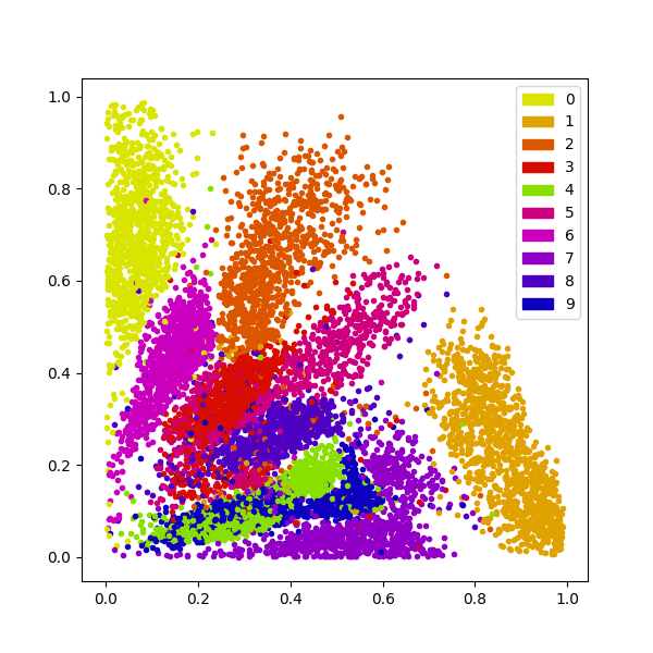
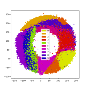
Scatter plot for the 2-dimension manifold is seen below. Note that code of the same digits tend to cluster in the latent space.

Plot

---

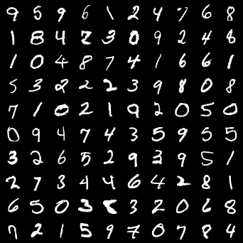
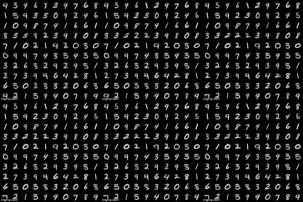
Below are the resonctruction results after 50 epochs with the sigmoid activation removed from the encoder.

Original	Reconstructed

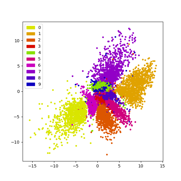
Scatter plot of the 2D manifold.

Plot

---

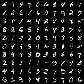
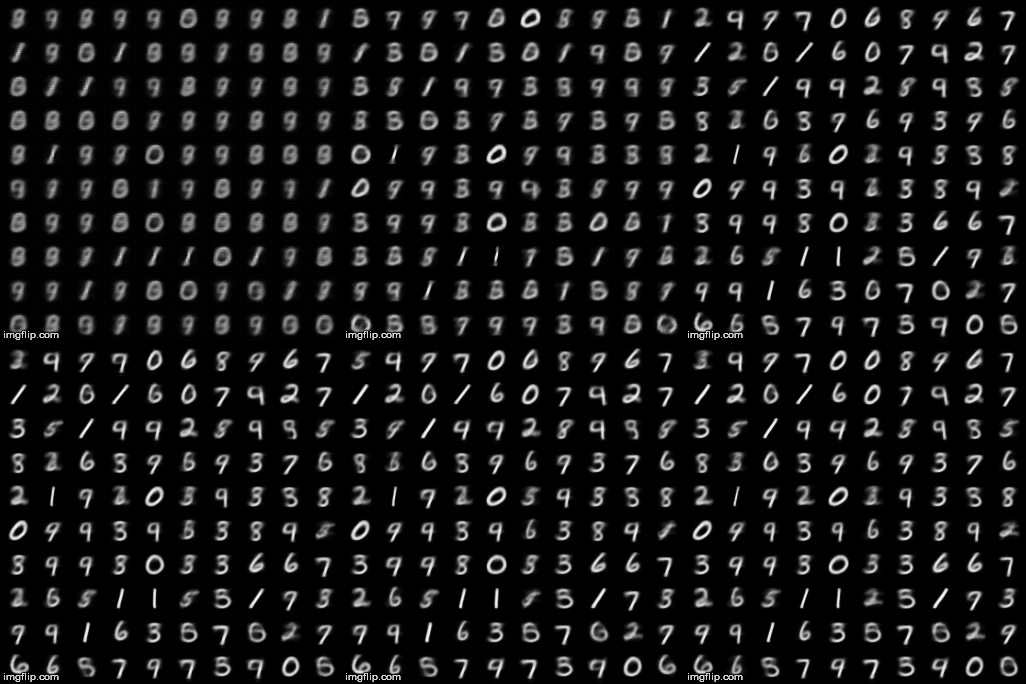
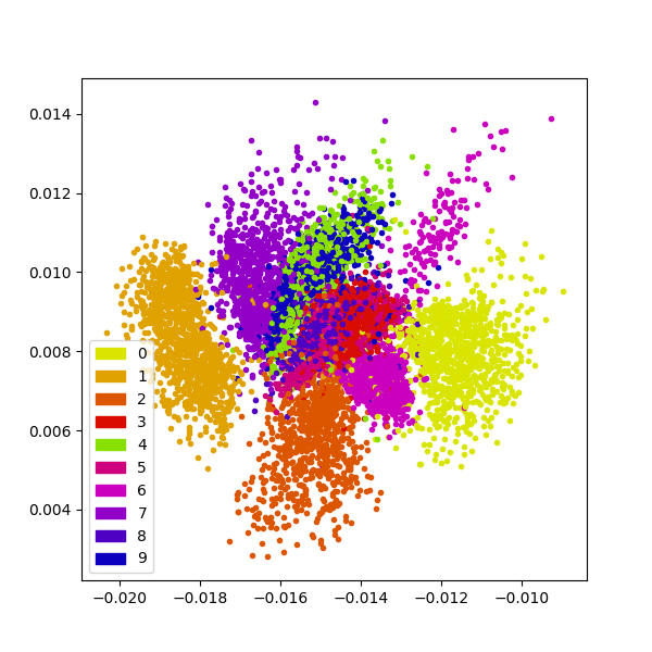
After adding L2 regularization of the latent codes to the loss (weight = 0.2), we can see the codes are restricted around to a small region.

Original	Reconstructed

Scatter plot of the 2D manifold.

Plot

---

---

[ VAE: Variational Autoencoder ]

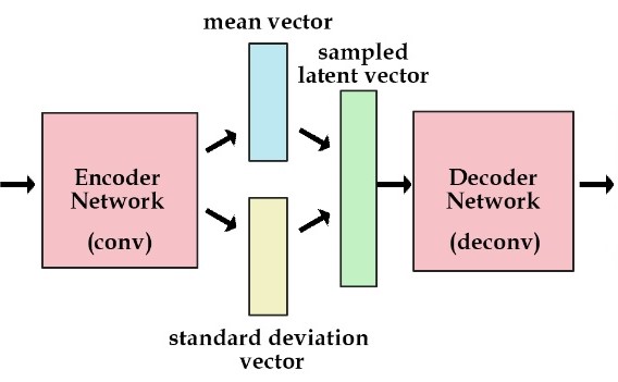
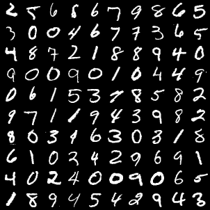
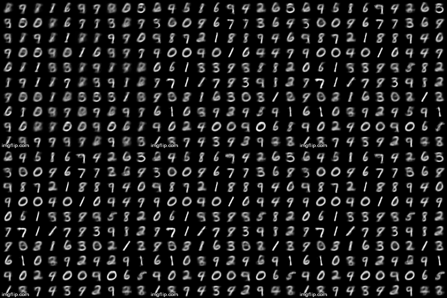
Unlike autoencoders, VAE encoders output two vectors, mean and sigma. We then sample from the normal distribution characterized by mean and sigma (let this distribution be Q), and take this as the decoder input.

Structure

In my experiment, a simple fully connected network is used.

 784 -> 400 -> (mu: 2, logvar: 2) -> 2 -> 400 -> 784

The numbers indicates the size of the hidden layer.

Objective

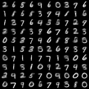
Usually the decoder input is sampled from a N(0,1) normal distribution. We can simply add a KL divergence loss between N, Q to the original autoencoder reconstruction loss so as to match Q with the desired N distribution.

Results

Original	Reconstructed	Random Generation

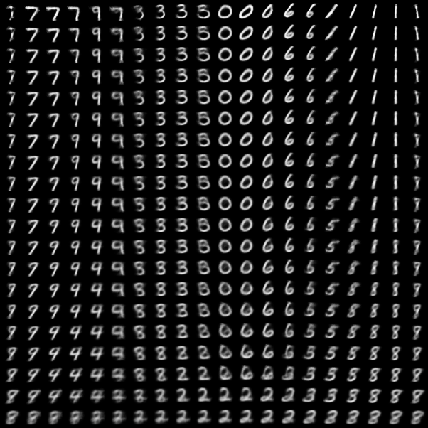
By sampling from uniform(0, 1) and transfroming it to Gaussian through Box-Muller method, we can visualize the 2-D continuous manifold.

Manifold

---

---

[ GAN: Generative Adversarial Networks ]

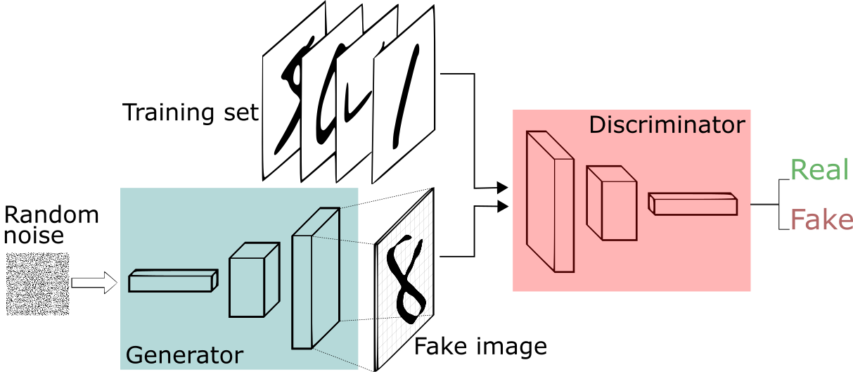
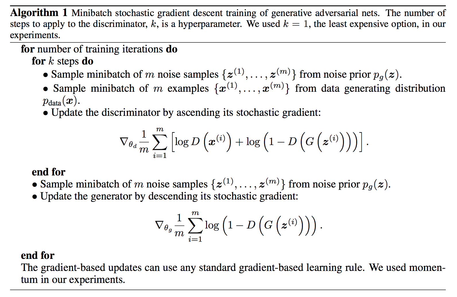
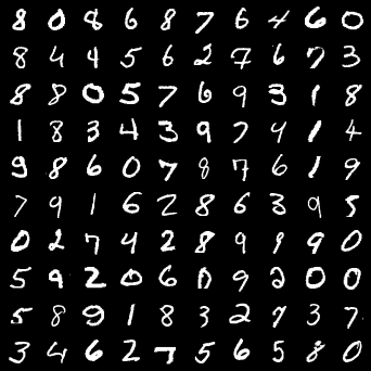
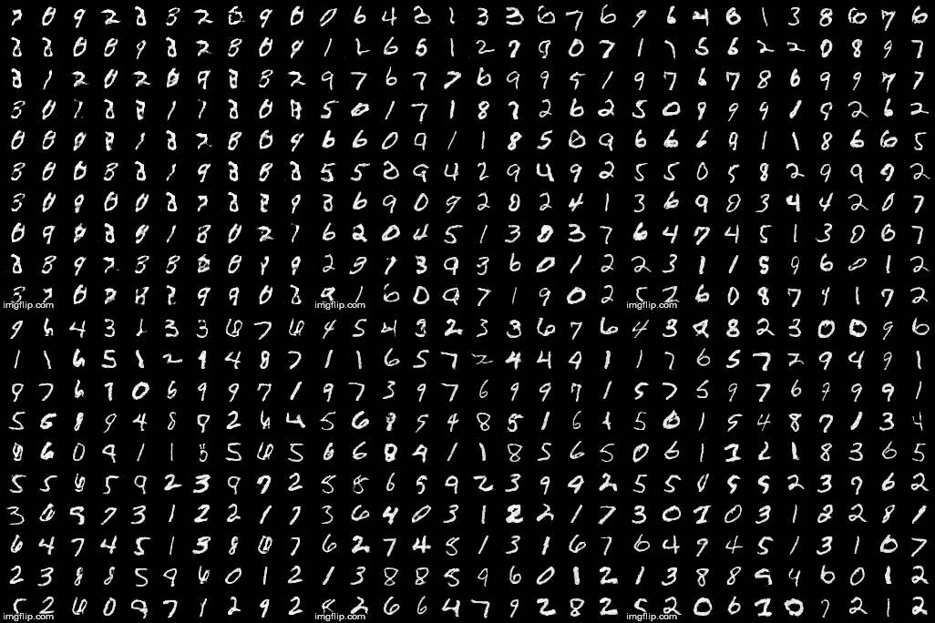
The groundwork for most generative models today, GANs are generally composed of two actors, a Generator and a Discriminator, who play a zero-sum game. The discriminator tries to distinguish real and synthesized images, while the generator learns to create images that fool the discriminator.

Structure

Algorithm

Results

Real images	Generated

---

---

[ Adversarial Autoencoders ]

Similar to VAE(Variational Autoencoders), the encoder in Adversairal Autoencoders (AAE) also learns to fit a given prior distribution, but by fooling a distribution discriminator rather tha n minimizing the KL divergence.

Structure

The discriminator tries to determine if the input is from a prior distribution p(z) or is generated by the decoder.

I simply employed the fully connected network setting in the original paper. The output for the encoder network is linear activation since many distributions has infinite range.

Results

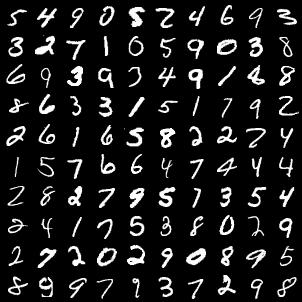
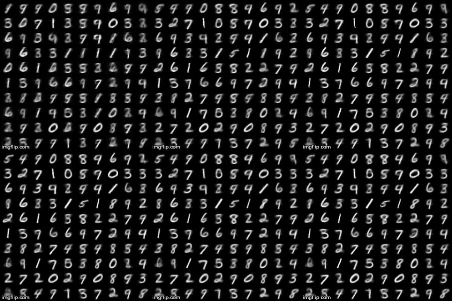
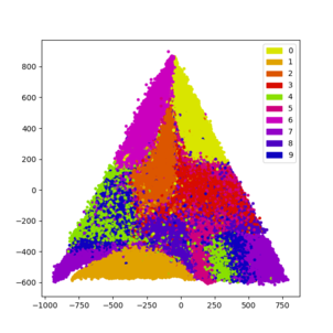
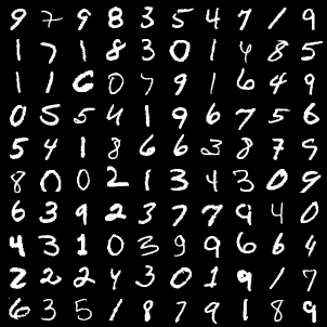
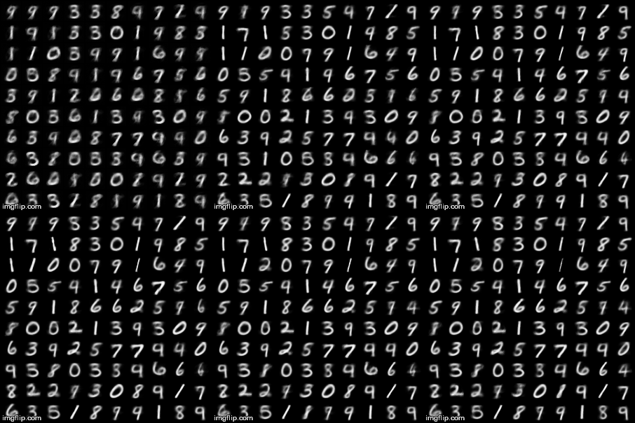
The encoder tries to fit a "triangle" and "donut" distribution. The results below show that the shape of the distribution is captured by the encoder.

Original	Reconstructed	Manifold

---

---

[ WGAN: Wasserstein's GAN ]

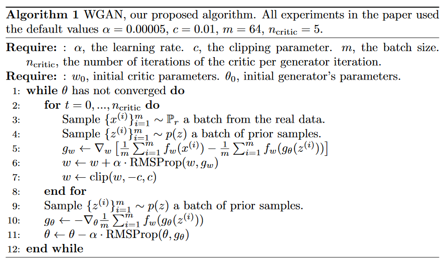
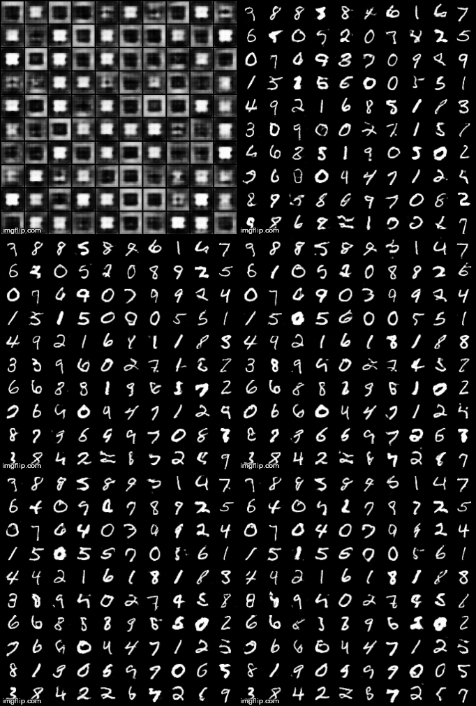
An (allegedly) more stable GAN model. Rather than minimizing the JS divergence between the prior training dats distribution and the generated data distribution as in GAN, WGAN minimizes the Wasserstein's distance.

Algorithm

Results

Real images	Generated

---

---

[ WGAN-GP: WGAN with Gradient Penalty ]

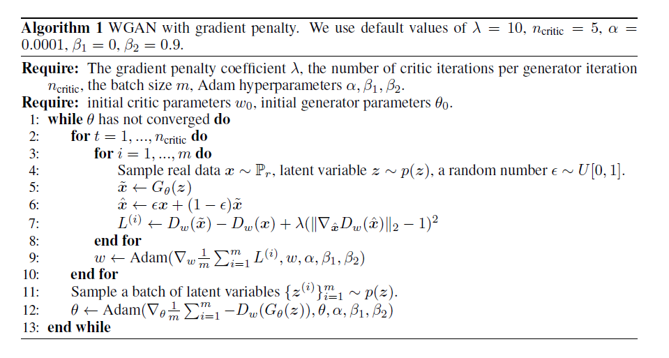
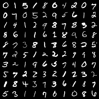
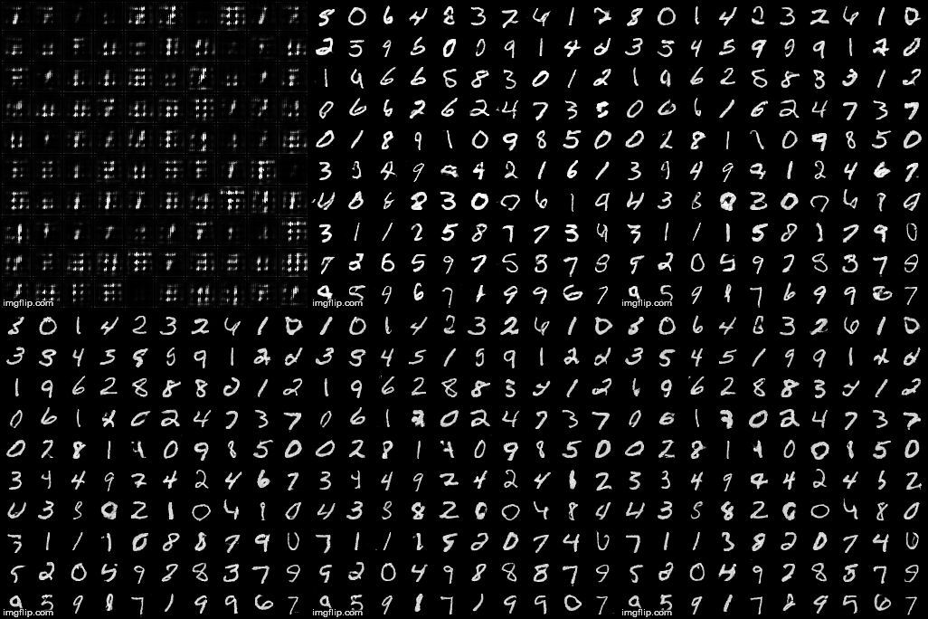
In WGAN, it is difficult to enforce the Lipschitz constraint. The original paper suggests clipping weights, but bad choices of the bounds may lead to failures. WGANGP resolves this problem by using gradient penalty to enforce the Lipshitz constraint.

Algorithm

Results

Real images	Generated

---

---

[ LSGAN: Least Squares GAN ]

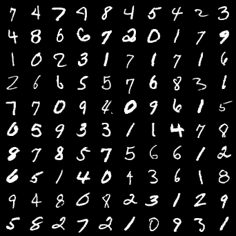
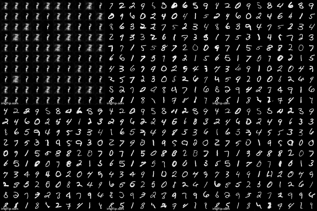
Yet another GAN variant with a modified loss function. Sigmoid activation is removed from the output layer of the discriminator, and we aim to minimize the L2 distance between the discriminator outputs and the wished score for each image.

Objective

a, b, c are hyperparameters to be determined (the scores we want fake and real images to have). In the original paper, the author uses a = 1, b = 0, c = 1.

Results

Real images	Generated

---

---

[ ACGAN: Auxiliary Classifier GANs ]

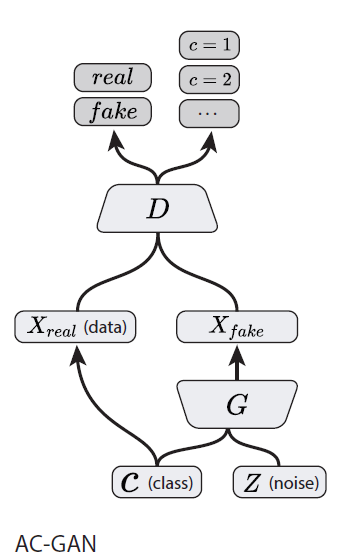
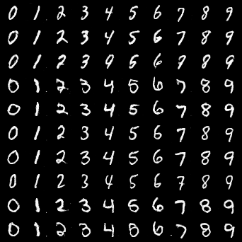
In ACGAN, the discriminator not only learns to distinguish fake and real images, but also tries to classify the image into correct labels. We can then manipulate the disentangled latent code and generate images conditioned on their class.

Structure

The class information is usually representated by a one-hot encoding. It is then concatenated with a noise vector and fed to the generator.

Objective

Results

Fixing noise	Generated

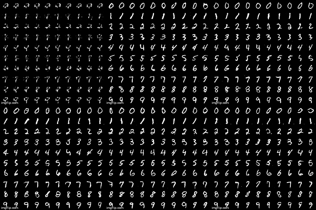When we fix the noise vector and only change the class label vector, ACGAN generates images from different classes but similar overall structure (eg. thickness, tilt, rotation...).

---

---

[ Conditional GAN ]

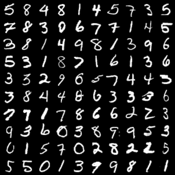
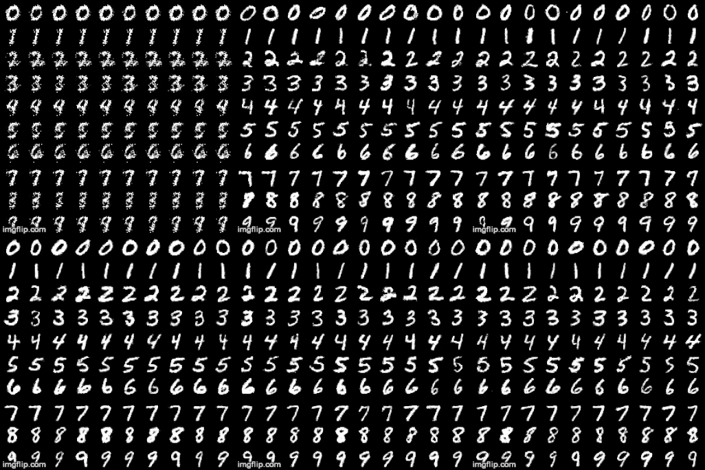
By simply providing extra information (eg. class labels) to both the discriminator and generator, we can extend the original GAN model to a conditional setting. That is, the generator would be able to perform conditional generation.

Struture

The conditional information can come in many forms. For simple multi-class labels, usually we just feed the networks with one-hot encodings. For more complex conditions such as text, we can train a better embedding (eg. word2vec), and the embedded code will be our condition.

Objective

Note that the loss is nearly identical to the original GAN loss, only that it is conditioned on some prior knowledge y.

Results

Real	Generated