An introduction to ML Fairness and Scikit-Learn

Summary
Analysis set-up
The data
Data prep
Exploration
Machine learning analysis
Bias mitigation via preprocessing
Bias mitigation via inprocessing
End

Summary

Welcome! The purpose of this notebook is to outline a very simple process for identifying and mitigating machine learning bias using fairlearn and imbalanced-learn. This post will rely on tried-and-true scikit learn best practices, so my hope is that it not only displays ways to handle potential bias issues, but also how to properly structure a basic supervised learning analysis. I am also experimenting with bias mitigation strategies provided by imbalanced-learn and fairlearn, so in the fairness assessment sections I am learning along with you! With that introduction, let's get into the data!

🚨 The axis labels on the plots are black, so if you're in GitHub Dark Mode, you will need to switch to Light Mode to view them!

Analysis set-up

# Imports

import warnings

warnings.filterwarnings('ignore')



import pandas as pd

import numpy as np

import pickle

import seaborn as sns

sns.set_style("white")

from fairlearn.metrics import MetricFrame, false_positive_rate, true_positive_rate, selection_rate, count, demographic_parity_ratio, equalized_odds_ratio

%matplotlib inline



from sklearn.preprocessing import OneHotEncoder, StandardScaler

from sklearn.model_selection import train_test_split

from sklearn.metrics import f1_score, accuracy_score, precision_score, recall_score

from sklearn.pipeline import Pipeline

from sklearn.svm import LinearSVC, SVC

from sklearn.neighbors import KNeighborsClassifier

from sklearn.linear_model import LogisticRegressionCV, LogisticRegression, SGDClassifier

from sklearn.ensemble import BaggingClassifier, ExtraTreesClassifier, RandomForestClassifier

The data

The data used in this analysis come from the UCI Machine Learning Repository (https://archive.ics.uci.edu/ml/datasets/default+of+credit+card+clients). It represents Taiwanese credit card clients. Our goal will be to predict who is at risk of defaulting on their credit card payment next month, indicated by the variable default payment next month.

The data include 23 variables:

X1: Amount of the given credit (NT dollar): it includes both the individual consumer credit and his/her family (supplementary) credit.
X2: Gender (1 = male; 2 = female).
X3: Education (1 = graduate school; 2 = university; 3 = high school; 4 = others).
X4: Marital status (1 = married; 2 = single; 3 = others).
X5: Age (year).
X6 - X11: History of past payment. We tracked the past monthly payment records (from April to September, 2005) as follows: - X6 = the repayment status in September, 2005; X7 = the repayment status in August, 2005; . . .;X11 = the repayment status in April, 2005. The measurement scale for the repayment status is: -1 = pay duly; 1 = payment delay for one month; 2 = payment delay for two months; . . .; 8 = payment delay for eight months; 9 = payment delay for nine months and above.
X12-X17: Amount of bill statement (NT dollar). X12 = amount of bill statement in September, 2005; X13 = amount of bill statement in August, 2005; . . .; X17 = amount of bill statement in April, 2005.
X18-X23: Amount of previous payment (NT dollar). X18 = amount paid in September, 2005; X19 = amount paid in August, 2005; . . .;X23 = amount paid in April, 2005.

df = pd.read_excel("../data/default of credit card clients.xls", header = 1)

print(f"Number of rows: {df.shape[0]}\nNumber of columns: {df.shape[1]}")

Number of rows: 30000
Number of columns: 25

df.head()

.dataframe tbody tr th {
    vertical-align: top;
}

.dataframe thead th {
    text-align: right;
}

</style>

	ID	LIMIT_BAL	SEX	EDUCATION	MARRIAGE	AGE	PAY_0	PAY_2	PAY_3	PAY_4	...	BILL_AMT4	BILL_AMT5	BILL_AMT6	PAY_AMT1	PAY_AMT2	PAY_AMT3	PAY_AMT4	PAY_AMT5	PAY_AMT6	default payment next month
0	1	20000	2	2	1	24	2	2	-1	-1	...	0	0	0	0	689	0	0	0	0	1
1	2	120000	2	2	2	26	-1	2	0	0	...	3272	3455	3261	0	1000	1000	1000	0	2000	1
2	3	90000	2	2	2	34	0	0	0	0	...	14331	14948	15549	1518	1500	1000	1000	1000	5000	0
3	4	50000	2	2	1	37	0	0	0	0	...	28314	28959	29547	2000	2019	1200	1100	1069	1000	0
4	5	50000	1	2	1	57	-1	0	-1	0	...	20940	19146	19131	2000	36681	10000	9000	689	679	0

5 rows × 25 columns

df.describe()

.dataframe tbody tr th {
    vertical-align: top;
}

.dataframe thead th {
    text-align: right;
}

</style>

	ID	LIMIT_BAL	SEX	EDUCATION	MARRIAGE	AGE	PAY_0	PAY_2	PAY_3	PAY_4	...	BILL_AMT4	BILL_AMT5	BILL_AMT6	PAY_AMT1	PAY_AMT2	PAY_AMT3	PAY_AMT4	PAY_AMT5	PAY_AMT6	default payment next month
count	30000.000000	30000.000000	30000.000000	30000.000000	30000.000000	30000.000000	30000.000000	30000.000000	30000.000000	30000.000000	...	30000.000000	30000.000000	30000.000000	30000.000000	3.000000e+04	30000.00000	30000.000000	30000.000000	30000.000000	30000.000000
mean	15000.500000	167484.322667	1.603733	1.853133	1.551867	35.485500	-0.016700	-0.133767	-0.166200	-0.220667	...	43262.948967	40311.400967	38871.760400	5663.580500	5.921163e+03	5225.68150	4826.076867	4799.387633	5215.502567	0.221200
std	8660.398374	129747.661567	0.489129	0.790349	0.521970	9.217904	1.123802	1.197186	1.196868	1.169139	...	64332.856134	60797.155770	59554.107537	16563.280354	2.304087e+04	17606.96147	15666.159744	15278.305679	17777.465775	0.415062
min	1.000000	10000.000000	1.000000	0.000000	0.000000	21.000000	-2.000000	-2.000000	-2.000000	-2.000000	...	-170000.000000	-81334.000000	-339603.000000	0.000000	0.000000e+00	0.00000	0.000000	0.000000	0.000000	0.000000
25%	7500.750000	50000.000000	1.000000	1.000000	1.000000	28.000000	-1.000000	-1.000000	-1.000000	-1.000000	...	2326.750000	1763.000000	1256.000000	1000.000000	8.330000e+02	390.00000	296.000000	252.500000	117.750000	0.000000
50%	15000.500000	140000.000000	2.000000	2.000000	2.000000	34.000000	0.000000	0.000000	0.000000	0.000000	...	19052.000000	18104.500000	17071.000000	2100.000000	2.009000e+03	1800.00000	1500.000000	1500.000000	1500.000000	0.000000
75%	22500.250000	240000.000000	2.000000	2.000000	2.000000	41.000000	0.000000	0.000000	0.000000	0.000000	...	54506.000000	50190.500000	49198.250000	5006.000000	5.000000e+03	4505.00000	4013.250000	4031.500000	4000.000000	0.000000
max	30000.000000	1000000.000000	2.000000	6.000000	3.000000	79.000000	8.000000	8.000000	8.000000	8.000000	...	891586.000000	927171.000000	961664.000000	873552.000000	1.684259e+06	896040.00000	621000.000000	426529.000000	528666.000000	1.000000

8 rows × 25 columns

df.dtypes

ID                            int64
LIMIT_BAL                     int64
SEX                           int64
EDUCATION                     int64
MARRIAGE                      int64
AGE                           int64
PAY_0                         int64
PAY_2                         int64
PAY_3                         int64
PAY_4                         int64
PAY_5                         int64
PAY_6                         int64
BILL_AMT1                     int64
BILL_AMT2                     int64
BILL_AMT3                     int64
BILL_AMT4                     int64
BILL_AMT5                     int64
BILL_AMT6                     int64
PAY_AMT1                      int64
PAY_AMT2                      int64
PAY_AMT3                      int64
PAY_AMT4                      int64
PAY_AMT5                      int64
PAY_AMT6                      int64
default payment next month    int64
dtype: object

Data prep

Before we can do any machine learning modelling, we first need to prepare the data for analysis. It's not ready in its current form! In the cells below, I walk through various feature engineering steps, including:

Checking whether any rows have missing values and mitigate as-needed
Generating binary representations of the categorical variables
Mapping the education column to a label representation
Zeroing out values less than 0 in strictly positive numerical categories
Changing the int-coded variables to pd.numeric types
One-hot encoding the education variable using pd.get_dummies

[(col, df[col].isnull().mean()) for col in df.columns.tolist()] #no missing values!

[('ID', 0.0),
 ('LIMIT_BAL', 0.0),
 ('SEX', 0.0),
 ('EDUCATION', 0.0),
 ('MARRIAGE', 0.0),
 ('AGE', 0.0),
 ('PAY_0', 0.0),
 ('PAY_2', 0.0),
 ('PAY_3', 0.0),
 ('PAY_4', 0.0),
 ('PAY_5', 0.0),
 ('PAY_6', 0.0),
 ('BILL_AMT1', 0.0),
 ('BILL_AMT2', 0.0),
 ('BILL_AMT3', 0.0),
 ('BILL_AMT4', 0.0),
 ('BILL_AMT5', 0.0),
 ('BILL_AMT6', 0.0),
 ('PAY_AMT1', 0.0),
 ('PAY_AMT2', 0.0),
 ('PAY_AMT3', 0.0),
 ('PAY_AMT4', 0.0),
 ('PAY_AMT5', 0.0),
 ('PAY_AMT6', 0.0),
 ('default payment next month', 0.0)]

df["male"] = np.where(df.SEX == 1, 1, 0)

df["under30"] = np.where(df.AGE < 30, 1, 0)

df["unmarried"] = np.where(df.MARRIAGE ==2, 1, 0)

df.rename(columns = {'default payment next month':'y'}, inplace = True)



educ_dict = {"EDUCATION": ["1", "2", "3", "4"], "EDUC_LEVEL": ["graduate_school", "university", "high_school", "other"]}

df["EDUCATION"] = df.EDUCATION.astype(str)

df = pd.merge(df, pd.DataFrame(educ_dict), on = "EDUCATION")



for col in ['PAY_0','PAY_2', 'PAY_3', 'PAY_4', 'PAY_5', 'PAY_6']:

    df.loc[df[col] < 0, col] = 0

for col in ['LIMIT_BAL', 'PAY_0', 'PAY_2', 'PAY_3', 'PAY_4', 'PAY_5', 'PAY_6',

       'BILL_AMT1', 'BILL_AMT2', 'BILL_AMT3', 'BILL_AMT4', 'BILL_AMT5',

       'BILL_AMT6', 'PAY_AMT1', 'PAY_AMT2', 'PAY_AMT3', 'PAY_AMT4', 'PAY_AMT5',

       'PAY_AMT6']: # int type columns

    df[col] = df[col].astype(float)



df = pd.get_dummies(df, prefix = "educ_", columns = ["EDUC_LEVEL"], drop_first = True)

Exploration

Now that the data is prepped, let's view how the distribution of our target variable changes across classes. Of particular interest to me are the SEX, Under 30, and Unmarried columns, as those could all be potentially encoding historical biases.

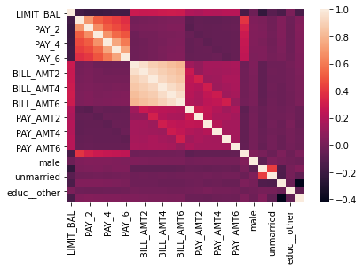
# Observing pairwise correlations; most of the variables (outside of the bill amounts) are not correlated.

corr = df.drop(columns = ["SEX", "AGE", "MARRIAGE", "ID", "EDUCATION"], axis = 1).corr()

sns.heatmap(corr)

<AxesSubplot:>

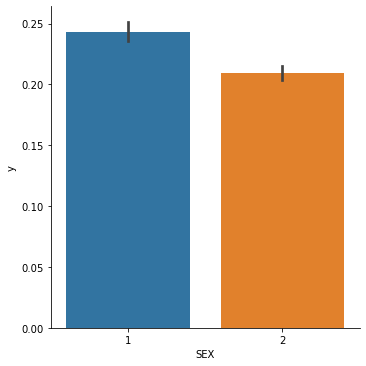
# NOTE: Sex = 1 if MALE and 2 if FEMALE

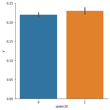
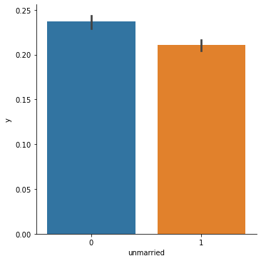
for col in ["SEX", "under30", "unmarried"]:

    sns.catplot(x = col, y = "y",  kind="bar", data = df)

The catplots above show the following results:

Women default on their credit card payments less frequently than men do
Credit card holders under age 30 default on their payments slightly more frequently than those over 30 do
Unmarried individuals default on their payments slightly less than married individuals do

Our classification model is going to pick up on these trends and use them to predict the likelihood of defaulting on a payment. The only result that looks slightly suspicious to me is that younger credit card holders default on their payments more often. My worry is that the model may reflect this reality by classifying younger folks are more likely to default, even when that isn't the case! Let's move on to the modelling stage to see if that happens.

Machine learning analysis

A priori, I don't know which classification model is going to give me the best fit. So the strategy I am going to take instead of fitting different models one-by-one is running a pipeline fit through a series of popular classifiers in an automated fashion. I'm going to use a loop to perform the following steps:

Create a pipeline with the steps Standard Scalar (scale the numerical features to have a standard normal distribution) and fitting a classifier
Split the data into train and test sets
Fit the pipeline to the training data
Generate the predicted values
Return the F1 score, which is the harmonic mean of the precision and the recall

All the results will be appended to the scores list, and I'll show you which ones performed the best (by the accuracy score, that is!)

# Dropping the old variables that we recoded earlier

X = df.drop(columns = ["SEX", "AGE", "MARRIAGE", "ID", "EDUCATION", "y"], axis = 1)

y = df.y

# define the models we want to test

models = [

    SVC(gamma='auto'), LinearSVC(),

    SGDClassifier(max_iter=100, tol=1e-3), KNeighborsClassifier(),

    LogisticRegression(solver='lbfgs'), LogisticRegressionCV(cv=3),

    BaggingClassifier(), ExtraTreesClassifier(n_estimators=300),

    RandomForestClassifier(n_estimators=300)

]



scores = []



# run models

for estimator in models:

    

    # pipeline

    pipe = Pipeline([

        ('scaler', StandardScaler(with_mean=False)),

        ('estimator', estimator)

    ])



    X_train, X_test, y_train, y_test = train_test_split(X, y, random_state=0)

    

    # Fit models

    pipe.fit(X_train, y_train)

    

    # Generate predictions

    expected = y_test

    predicted = pipe.predict(X_test)

    score = f1_score(y_true = expected, y_pred = predicted)



    # Compute and return F1 (harmonic mean of precision and recall)

    scores.append((estimator.__class__.__name__, score) )



print(sorted(scores, key = lambda s: s[1], reverse= True))

[('SGDClassifier', 0.5058651026392962), ('RandomForestClassifier', 0.4682170542635659), ('SVC', 0.4653584301161394), ('ExtraTreesClassifier', 0.4578768417075935), ('BaggingClassifier', 0.4407045009784736), ('LogisticRegression', 0.4395243952439525), ('LogisticRegressionCV', 0.4395243952439525), ('LinearSVC', 0.4269568857262453), ('KNeighborsClassifier', 0.41973490427098675)]

So the best classifier by accuracy is the SDGclassifier, which implements a regularized linear models with stochastic gradient descent (SGD) learning. It achieves a F1 score of about 50%. That's not great! Let's see how the evaluation metrics break down across the attributes we deemed as sensitive.

pipe = Pipeline([ 

    ('scaler', StandardScaler(with_mean=False)), 

    ('estimator', SGDClassifier(max_iter=100, tol=1e-3) ) 

    ])



X_train, X_test, y_train, y_test = train_test_split(X, y, random_state=0)



pipe.fit(X_train, y_train)

    

expected = y_test

predicted = pipe.predict(X_test)



metrics = {

    'accuracy': accuracy_score,

    'precision': precision_score,

    'recall': recall_score,

    'false positive rate': false_positive_rate,

    'true positive rate': true_positive_rate,

    'selection rate': selection_rate,

    'count': count}

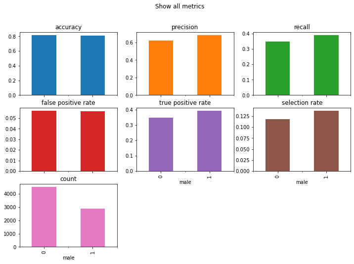
Let's start by assessing parity across gender. We'll review how the model performs across a variety of different evaluation metrics for each gender.

gender_frame = MetricFrame(metrics=metrics, y_true=expected, y_pred=predicted, sensitive_features=X_test["male"])

print(gender_frame.by_group)



gender_frame.by_group.plot.bar(

    subplots=True,

    layout=[3, 3],

    legend=False,

    figsize=[12, 8],

    title="Show all metrics",

)

      accuracy precision    recall false positive rate true positive rate  \
male                                                                        
0     0.808159  0.696682   0.15425            0.017867            0.15425   
1     0.781869  0.742424  0.141618            0.015546           0.141618   

     selection rate count  
male                       
0          0.046527  4535  
1          0.045849  2879  





array([[<AxesSubplot:title={'center':'accuracy'}, xlabel='male'>,
        <AxesSubplot:title={'center':'precision'}, xlabel='male'>,
        <AxesSubplot:title={'center':'recall'}, xlabel='male'>],
       [<AxesSubplot:title={'center':'false positive rate'}, xlabel='male'>,
        <AxesSubplot:title={'center':'true positive rate'}, xlabel='male'>,
        <AxesSubplot:title={'center':'selection rate'}, xlabel='male'>],
       [<AxesSubplot:title={'center':'count'}, xlabel='male'>,
        <AxesSubplot:xlabel='male'>, <AxesSubplot:xlabel='male'>]],
      dtype=object)

Okay, so as you can see above, the model is slightly likelier to classify women as defaulting on a payment even when in reality they did not (false positive class). The selection rate, or percentage of the population which have ‘1’ as their label, is roughly equal across groups. Let's also look at the few boilerplate fair ML classification metrics.

# Demographic parity ratio is defined as the ratio between the smallest and the largest group-level selection rate across all sensitive attributes

# The closer to 1, the better!

d = demographic_parity_ratio(y_true=expected, y_pred=predicted, sensitive_features=X_test["male"])



# Equalized odds ratio is defined as the smaller of two metrics: true_positive_rate_ratio and false_positive_rate_ratio

# The closer to 1, the better!

e = equalized_odds_ratio(y_true=expected, y_pred=predicted, sensitive_features=X_test["male"])



print(f"Demographic parity ratio: {d}\nEqualized odds ratio: {e}")

Demographic parity ratio: 0.9854330015194191
Equalized odds ratio: 0.8701131687242798

Both ratios are close to 1, which is pretty good! How does this analysis change for the under30 variable?

age_frame = MetricFrame(metrics=metrics, y_true=expected, y_pred=predicted, sensitive_features=X_test["under30"])

print(age_frame.by_group)



age_frame.by_group.plot.bar(

    subplots=True,

    layout=[3, 3],

    legend=False,

    figsize=[12, 8],

    title="Show all metrics",

)



d = demographic_parity_ratio(y_true=expected, y_pred=predicted, sensitive_features=X_test["under30"])

e = equalized_odds_ratio(y_true=expected, y_pred=predicted, sensitive_features=X_test["under30"])



print(f"Demographic parity ratio: {d}\nEqualized odds ratio: {e}")

         accuracy precision    recall false positive rate true positive rate  \
under30                                                                        
0        0.796831  0.735135  0.123636            0.012609           0.123636   
1        0.800247  0.689873       0.2            0.026022                0.2   

        selection rate count  
under30                       
0             0.037104  4986  
1             0.065074  2428  
Demographic parity ratio: 0.5701787790623873
Equalized odds ratio: 0.48455995882655684

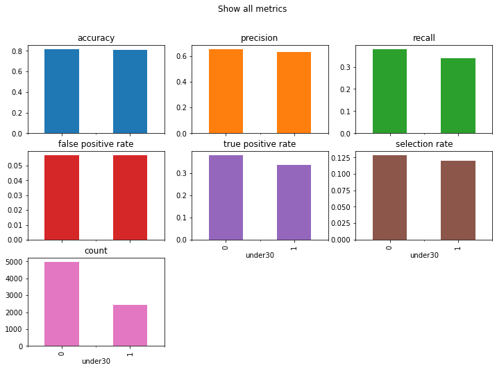
The fairness metrics are far worse for the under30 variable. Credit card holders under age 30 are erroneously predicted as likely to default (see the false positive rate). If you look at the count graph, you'll also see that there are way less observations for the under 30 group. One potential way to mitigate bias in our results is to reconstruct our dataset so that we have more representations of the minority group.

In a machine learning analysis, there are three places where bias mitigation can occur:

Preprocessing: Preprocessing involves identifying data gaps before the machine learning analysis begins. Typically, this can involve resampling/reweighting data to increase representation of underrepresented minority groups and feature engineering by modyfing the labels or label-data pairs.
In-processing: In-processing involes including a regularization parameter to a model to optimize the model for fairness while it's training.
Post-processing: Post-processing involves changing the thresholds of the evaluation metric you're using to incorporate fairness goals.

In an ideal world, bias mitigation would begin before machine learning starts. It's easier to achieve the goals of fairness AND accuracy, precision, AOC_RUC score, etc. if we reweight/resample the data before running a model. Why is this the case? Well, during in-processing, if you're trying to achieve an outcome while adhering to a fairness constraint, your outcome may be worse off than if the constraint was not there. Similarly, if you're adjusting the threshold of an evaluation metric to accomodate a fairness constraint, even if you get the metric to an acceptable level, that metric is reflective of the model's capability to pick up on signals in the data, and one signal is data bias. I've explained this before as garbage-in, garbage-out; even if you dress up the garbage you get from the model, that doesn't change the fact that garbage was used to produce it!

In the section below, I attempt to address the disparate outcomes for younger credit card holders using resampling.

Bias mitigation via preprocessing

from imblearn.over_sampling import SMOTE

from imblearn.pipeline import make_pipeline



# Redo the pipeline with the SMOTE parameter added in and reassess the results



pipe = make_pipeline(SMOTE(random_state=0), StandardScaler(with_mean=False), SGDClassifier(max_iter=100, tol=1e-3) )



X_train, X_test, y_train, y_test = train_test_split(X, y, random_state=0)

    

pipe.fit(X_train, y_train)



y_true = y_test

y_pred = pipe.predict(X_test)

age_frame = MetricFrame(metrics=metrics, y_true=y_true, y_pred=y_pred, sensitive_features=X_test["under30"])



age_frame.by_group.plot.bar(

    subplots=True,

    layout=[3, 3],

    legend=False,

    figsize=[12, 8],

    title="Show all metrics",

)



print(age_frame.by_group)



d = demographic_parity_ratio(y_true=y_true, y_pred=y_pred, sensitive_features=X_test["under30"])

e = equalized_odds_ratio(y_true=y_true, y_pred=y_pred, sensitive_features=X_test["under30"])

print(f"Demographic parity ratio: {d}\nEqualized odds ratio: {e}")

         accuracy precision    recall false positive rate true positive rate  \
under30                                                                        
0        0.754513  0.453172  0.545455             0.18631           0.545455   
1        0.793245  0.548975  0.442202            0.105151           0.442202   

        selection rate count  
under30                       
0             0.265544  4986  
1             0.180807  2428  
Demographic parity ratio: 0.6808949715554183
Equalized odds ratio: 0.5643897272191137

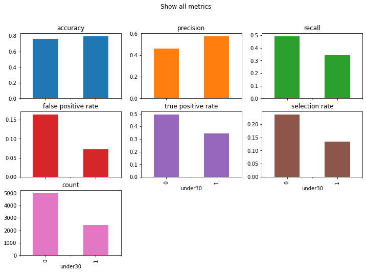
After applying SMOTE resampling, we can see that younger cardholders now have a lower false positive and lower selection rate than they did previously. The accuracy has fallen to slightly under 80%. The count reflects the underrepresentation in the original dataset and should be ignored. Because outcomes for the under-30 group are now better across the board, demographic parity and equalized odds suffer. In a more rigorous analysis, I'd experiment with other sampling and reweighting schemes to get as close to equal outcomes between groups as possible.

Bias mitigation via inprocessing

In the cell below, I apply an inprocessing method, a reduction (of the demographic parity flavor) to constrain the SVC classifier along a fairness requirement.

from fairlearn.reductions import ExponentiatedGradient, DemographicParity



dp = DemographicParity(difference_bound=0.01)

reduction = ExponentiatedGradient(SGDClassifier(max_iter=100, tol=1e-3), dp)

reduction.fit(X_train, y_train, sensitive_features=X_train["under30"])

y_pred = reduction.predict(X_test, random_state = 0)

age_frame = MetricFrame(metrics=metrics, y_true=y_test, y_pred=y_pred, sensitive_features=X_test["under30"])



print(age_frame.by_group)



d = demographic_parity_ratio(y_true=y_test, y_pred=y_pred, sensitive_features=X_test["under30"])

e = equalized_odds_ratio(y_true=y_test, y_pred=y_pred, sensitive_features=X_test["under30"])

print(f"Demographic parity ratio: {d}\nEqualized odds ratio: {e}")

         accuracy precision recall false positive rate true positive rate  \
under30                                                                     
0        0.779382       0.0    0.0                 0.0                0.0   
1        0.775535       0.0    0.0                 0.0                0.0   

        selection rate count  
under30                       
0                  0.0  4986  
1                  0.0  2428  
Demographic parity ratio: nan
Equalized odds ratio: nan

As you can see in the results above, nearly every evaluation metric is zeroed out. Demographic parity and equalized odds are also missing. I'd consider these results to be unstable. If I wanted to improve precision and recall across both groups, I'd continue to toggle the DemographicParity() constraint until I attained satisfactory results. The fairlearn documentation notes that picking the appropriate evaluation metric constraint is crucial, and in a real-world situation, this is something that I or my team would have determined ahead of time in accordance with the project's goals.

In a more rigorous analysis, I'd also do a grid search on the hyperparameters of the SDG classifier to ensure I got the best fit.

End

Thank you for reading 😄. If you'd like to learn more about ML fairness, check out my presentation on the topic and the the fairlearn documentation!

alliesaizan / classification-bias-experiment