a-akram / trackml-100

Solution ranked #100 in the TrackML competition on Kaggle

TrackML 100^th place

This repository contains the solution ranked #100 in the private leaderboard of the TrackML competition on Kaggle.

Apparently, this solution performs particularly well at finding particles that do not come from the collision axis. Based on post-competition analysis, David Rousseau (one of the organizers) wrote:

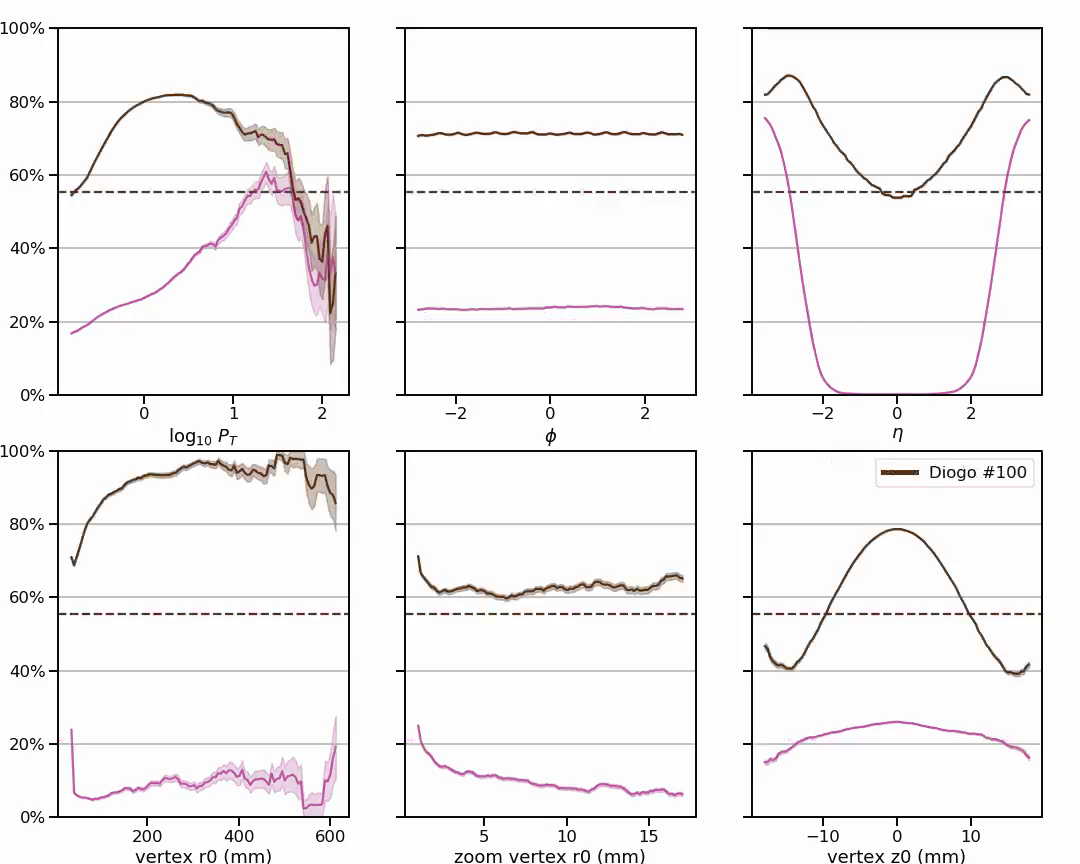
(the odd one out: in the bottom left plot, one can briefly see a dark curve rising high, this is Diogo's submission. It shows that his code finds particularly well particles that do NOT come from the z axis (axis of symmetry) (large r0), while most particles come from there (small r0), and most participants focus on particle with small r0, or even assume they come almost exactly from the z axis. Diogo's score is 0.55480, hardly better than the best public kernel, but his algorithm must be quite interesting)

Main idea

The training set contains on the order of 10⁴ events (event ids). Each event contains on the order of 10⁴ particles (particle ids). Therefore, there are a total of about (10⁴ events) * (10⁴ particles per event) = 10⁸ training particles.

Although there are many particles, the routes that these particles travel through space are constrained by the experimental setup and the laws of physics. For example, since there is a magnetic field, charged particles will have helical trajectories.

We could try to create a model that takes into account this particular experimental setup. We could even try to learn that model from the training data, and I guess many competitors have worked along these lines.

However, in this competition I tried a more general approach. Regardless of the particular experimental setup, I tried to answer the following question:

• Given a large amount of training particles, is it possible to do track reconstruction from test hits by finding the training particles that best fit the test hits?

To better explain this idea, consider the following picture:

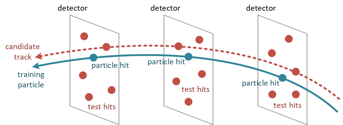
In the picture above, there is a training particle that passes through three detectors. In each of these detectors, there are multiple test hits. Some test hits will be closer to the training particle than others.

The main idea is to do the following:

• Pick the test hits that are closest to the particle hits on each detector. Calculate the average distance between the particle hits and their closest test hits across detectors.

• Repeat this process for every training particle. Get the closest test hit on each detector that the particle passes through. Calculate the average distance between particle hits and their closest test hits across detectors.

• For each training particle that is considered, there will be a candidate track comprising the test hits that are closest to that particle. This candidate track is characterized by a certain average distance.

• The best candidate tracks are the ones with the smallest average distances.

In the original dataset for the competition, every particle hit is associated with a certain weight. When computing the average distances, use a weighted average that takes these weights into account.

Using routes instead of particles

To reduce the computational burden and improve the results, we group particles that go through exactly the same sequence of detectors. These particles are said to have the same route.

In the picture below, we consider three detectors and four particles that pass through these (and only these) detectors in exactly the same sequence.

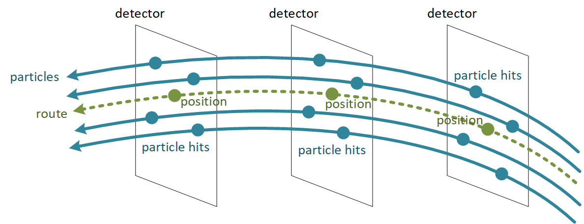
The route is calculated as the "mean trajectory" of these particles. At each detector, we calculate the mean position of the particle hits. The route is defined by the sequence of such positions across detectors.

To identify candidate tracks, we follow the same procedure as described above, but now using routes instead of the original particles, as illustrated in the following picture:

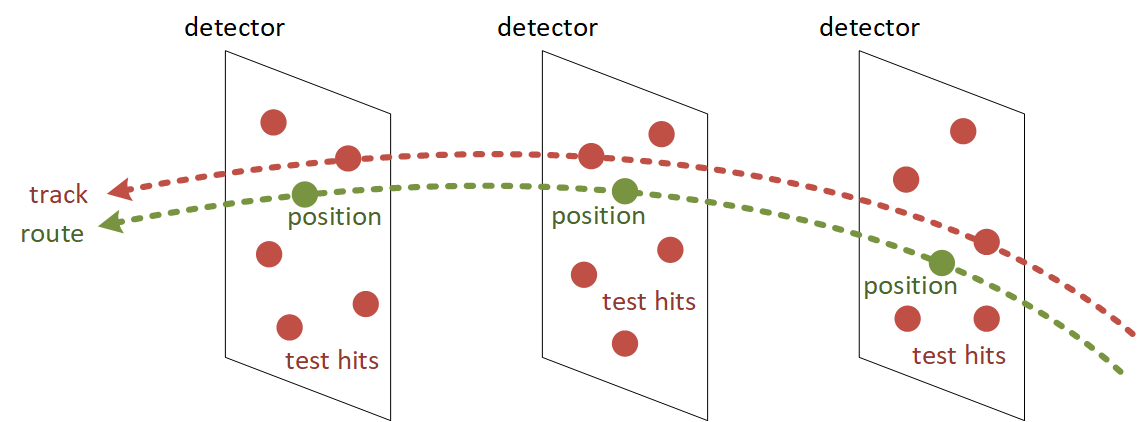
This means that only one candidate track will be considered for each unique sequence of detectors. However, different routes may share some detectors, so candidate tracks may compete for test hits on those detectors.

In general, better candidate tracks (i.e. the ones with smaller average distance) are given priority in picking their test hits. Other candidate tracks (with larger average distances) have to pick their test hits from the leftovers.

This could make some candidate tracks even worse, by slightly increasing their average distance. For simplicity, we do not update the average distances for tracks. Decisions are based on the average distances that were calculated initially.

The solution in 3 steps

1. The first step is particles: it comprises qsub_particles.py, particles.py and merge_particles.py.

2. The second step is routes: it comprises qsub_routes.py, routes.py.

3. The third step is tracks: it comprises qsub_tracks.py, tracks.py and merge_tracks.py.

The first step: particles

The core of this step is particles.py. For a given event id (or set of event ids), this script reads and joins the hits file and the truth file for that event (event*-hits.csv and event*-truth.csv).

Random hits are discarded (those with particle id equal to zero).

All particle ids (within an event) are renumbered sequentially, starting from 1.

A detector id is built by concatenating the volume id, layer id and module id for each hit.

The hits for each event are sorted by particle id and then by absolute value of z.

The x,y,z position of each hit is normalized by the distance to the origin. (This will be important when calculating average distances, because distances far away from the origin could be much larger than distances close to the origin.)

The end result - in the form of a list of hits with event id, particle id, detector id, normalized x,y,z and weight - is saved to a CSV file (event*-particles.csv).

What is qsub_particles.py?

qsub_particles.py is a script to distribute the execution particles.py on a PBS cluster.

Basically, it sets up n workers by distributing the event ids in a round-robin fashion across these workers.

Each worker runs particles.py with the event ids that have been assigned to it.

In case the execution is interrupted or some workers fail, qsub_particles.py will check which event ids are missing and will again launch n workers to handle those missing events.

What is merge_particles.py?

Since the events are processed independently, there is a final step to merge all processed events (i.e. the output files event*-particles.csv) into a single CSV file (which will be called particles.csv).

As a result of this step, we will have a particles.csv file of about 48.0 GB.

The second step: routes

The core of this step is routes.py. This script reads the output file from the previous step (particles.csv) into memory. (Yes, it reads 48 GB into RAM. I tried using Dask to avoid this, but at the time of this competition, Dask did not support the aggregations that will be computed next.)

The x,y,z positions of each hit are brought together into a new column named position.

The hits are grouped by particle id, and the following aggregations are performed:

• For each particle id, we create a sequence of detector ids that the particle goes through (see above for the definition of detector id).

• For each particle id, we create a sequence of positions that the particle goes through (based on the new position column that we just defined).

• For each particle id, we also keep the sequence of weights that correspond to the particle hits (see the dataset description for a definition of weight).

Now that hits are grouped by particle, we will group particles by sequence of detectors (route):

• For each sequence of detector ids, we group all the particles that have traveled through that sequence of detectors. The hit positions are stored in a 2D array where each row represents a different particle and each column represents a different detector.

• The corresponding hit weights are also stored in a 2D array.

Now, we are not going to keep multiple particles for each sequence of detectors. Instead, our goal is to keep only the "mean trajectory" of the particles that have traveled across the same route.

For this purpose:

• We calculate the count of particles that have traveled across each route.

• We calculate the mean position of the particle hits at each detector, along each route.

• We calculate the mean weight of the particle hits at each detector, along each route.

The end result - in the form of a list of routes with detector sequence, particle count, position sequence and weight sequence - is saved to a CSV file (event*-particles.csv).

The routes are sorted by count in descending order, so that routes traveled by the largest number of particles will be considered first in the next step.

What is qsub_routes.py?

Nothing special. Just the command that runs routes.py as a single worker on a PBS cluster.

Note, however, the memory requirement: 500 GB of RAM. (Again, it might be possible to alleviate this requirement, and significantly accelerate the computation time, by using Dask.)

As a result of this second step, we will have a routes.csv file of about 23.5 GB.

The third step: tracks

The core of this step is tracks.py. For a given test event, this script reads the corresponding hits file (event*-hits.csv).

• In a similar way to particles.py, it builds a detector id by concatenating the volume id, layer id and module id for each hit. It also normalizes the x,y,z position of each hit by the distance to the origin.

• In a similar way to routes.py, the x,y,z position of each test hit is brought into a new column named position.

The test hits are grouped by detector id. For each detector id, we have a list of test hit ids, and another list with their positions.

Subsequently, we read routes.csv that was created in the previous step. We go through this file line by line, where each line corresponds to a different route.

For each route being considered, we go through the detector sequence in order to pick the best hits, i.e. the test hits that are closest to the route position at each detector.

We then calculate the weighted average distance between those test hits and the route positions across detectors.

Some computational shortcuts when iterating through all the routes:

• Since routes have been sorted in descending order of particle count, when we get to routes that have been traveled by a single particle, we simply discard those routes and stop reading routes.csv. The rationale for doing this is that these could be random, one-of-a-kind routes that are not worth considering.

• There is no point in considering routes whose weights are all zero, so we skip these routes as well, in case they appear.

• Only those routes for which there are test hits in every detector along that route should be considered. If there are no test hits in some detector along the route, we skip that route.

After iterating through routes, we sort them by average distance. Routes with lower average distance will be listed first, as these seem to be a better fit to the test hits.

Test hits are then assigned to routes on a first-come, first-served basis. Since the best-fitting routes are listed first, these can pick the test hits that best suit them. The remaining routes will have to pick test hits from the leftovers.

The test hits that have been picked by a route are assigned the same track id. (A new track id is generated for each route.) Any test hits that are left unpicked by routes are assigned a track id of zero.

The end result - in the form of a list of test hits with event id, hit id and track id - are saved to a CSV file (event*-tracks.csv).

What is qsub_tracks.py?

qsub_tracks.py is a script to distribute the execution tracks.py on a PBS cluster.

The test events are processed independently. Each event id is processed by a separate worker.

In case the execution is interrupted or some workers fail, qsub_tracks.py will check which event ids are missing and will launch workers to handle those missing events.

What is merge_tracks.py?

Since the test events are processed independently, there is a final step to merge all processed events (i.e. the output files event*-tracks.csv) into a single CSV file (which will be called tracks.csv).

As a result of this step, we will have a tracks.csv file of about 206.1 MB. This is the file that can be submitted to Kaggle.