Normalizing flows

Reimplementations of density estimation algorithms from:

Block Neural Autoregressive Flow

https://arxiv.org/abs/1904.04676

Implementation of BNAF on toy density estimation datasets.

Results

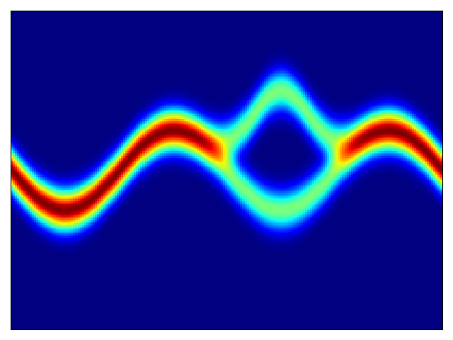
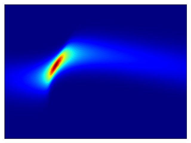
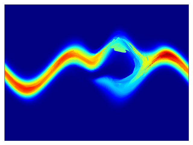
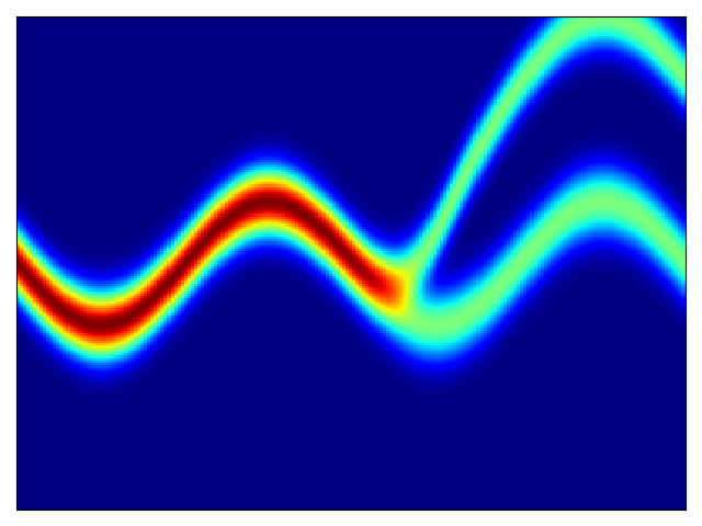
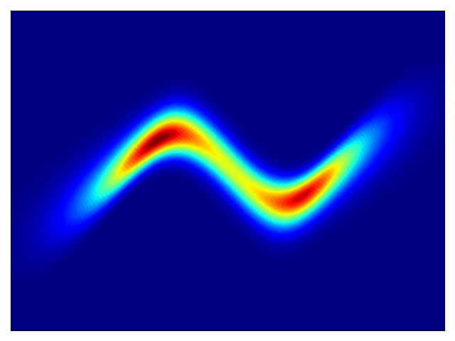
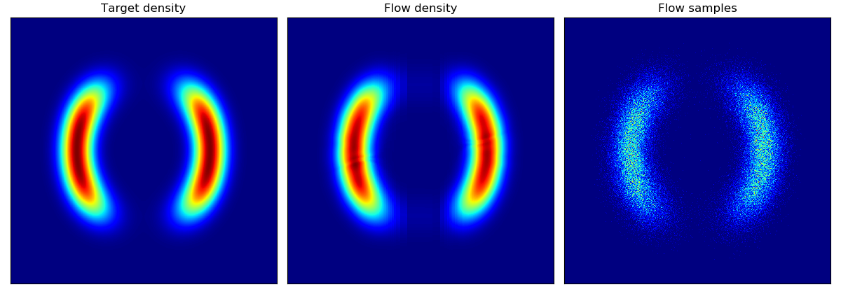
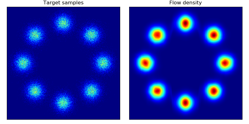
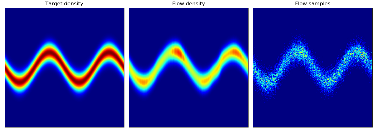
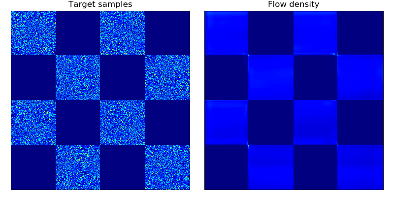
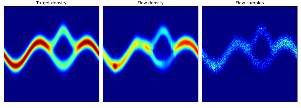
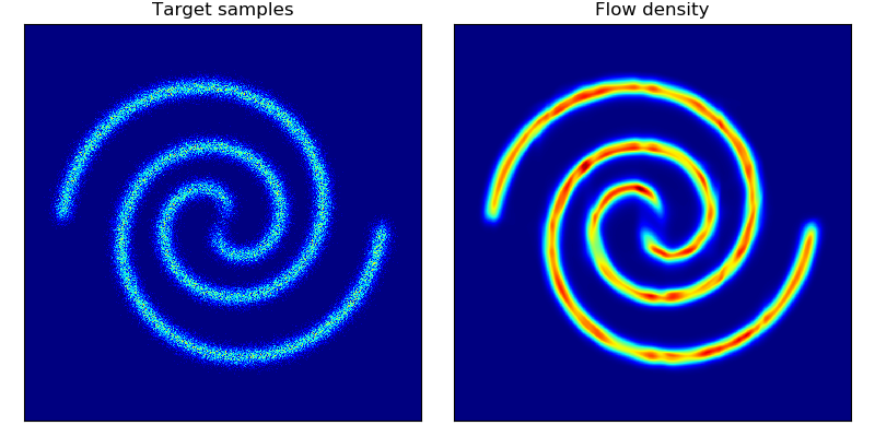
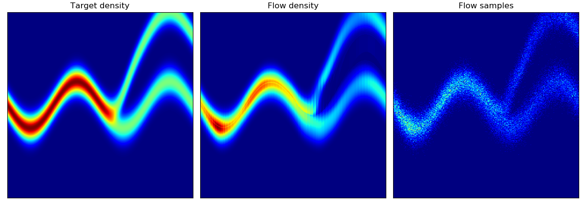
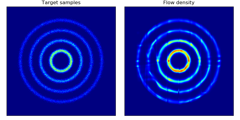
Density estimation of 2d toy data and density estimation of 2d test energy potentials (cf. Figure 2 & 3 in paper):

The models were trained for 20,000 steps with the architectures and hyperparameters described in the Section 5 of the paper, with the exception of rings dataset (bottom right) which had 5 hidden layers. The models trained significantly faster than the planar flow model in Rezende & Mohamed and were much more stable; interestingly, BNAF stretches space differently and requires a lot more test points to show a smooth potential.

Density matching on 2d energy potentials	Density estimation on 2d toy data

Usage

To train model:

python bnaf.py --train
               --dataset      # choice from u1, u2, u3, u4, 8gaussians, checkerboard, 2spirals
               --log_interval # how often to save the model and visualize results
               --n_steps      # number of training steps
               --n_hidden     # number of hidden layers
               --hidden_dim   # dimension of the hidden layer
               --[add'l options]

Additional options are: learning rate, learning rate decay and patience, cuda device id, batch_size.

To plot model:

python bnaf.py --plot
               --restore_file [path to .pt checkpoint]

Useful resources

Official implementation by the authors https://github.com/nicola-decao/BNAF

Glow: Generative Flow with Invertible 1x1 Convolutions

https://arxiv.org/abs/1807.03039

Implementation of Glow on CelebA and MNIST datasets.

Results

I trained two models:

Model A with 3 levels, 32 depth, 512 width (~74M parameters). Trained on 5 bit images, batch size of 16 per GPU over 100K iterations.
Model B with 3 levels, 24 depth, 256 width (~22M parameters). Trained on 4 bit images, batch size of 32 per GPU over 100K iterations.

In both cases, gradients were clipped at norm 50, learning rate was 1e-3 with linear warmup from 0 over 2 epochs. Both reached similar results and 4.2 bits/dim.

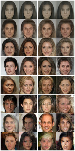
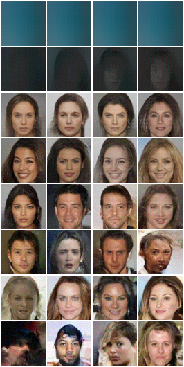
Samples at varying temperatures

Temperatures ranging 0, 0.25, 0.5, 0.6, 0.7, 0.8, 0.9, 1 (rows, top to bottom):

Model A	Model B

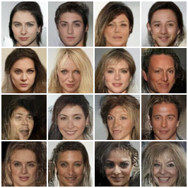
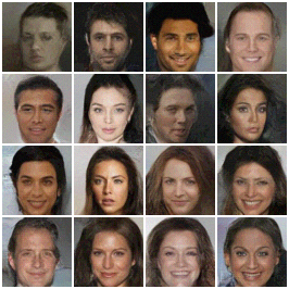
Samples at temperature 0.7:

Model A	Model B

Model A attribute manipulation on in-distribution sample:

Embedding vectors were calculated for the first 30K training images and positive / negative attributes were averaged then subtracting. The resulting dz was ranged and applied on a test set image (middle image represents the unchanged / actual data point).

Attribute	`dz` range [-2, -1, 0, 1, 2]
Brown hair
Male
Mouth slightly opened
Young

Model A attribute manipulation on 'out-of-distribution' sample (i.e. me):

Attribute	`dz` range
Brown hair
Mouth slightly opened

Usage

To train a model using pytorch distributed package:

python -m torch.distributed.launch --nproc_per_node=NUM_GPUS_YOU_HAVE \
       glow.py --train \
               --distributed \
               --dataset=celeba \
               --data_dir=[path to data source] \
               --n_levels=3 \
               --depth=32 \
               --width=512 \
               --batch_size=16 [this is per GPU]

For larger models or image sizes add --checkpoint_grads to checkpoint gradients using pytorch's library. I trained a 3 layer / 32 depth / 512 width model with batch size of 16 without gradient checkpointing and a 4 layer / 48 depth / 512 width model with batch size of 16 which had ~190M params so required gradient checkpointing (and was painfully slow on 8 GPUs).

To evaluate model:

python glow.py --evaluate \
               --restore_file=[path to .pt checkpoint] \
               --dataset=celeba \
               --data_dir=[path to data source] \
               --[options of the saved model: n_levels, depth, width, batch_size]

To generate samples from a trained model:

python glow.py --generate \
               --restore_file=[path to .pt checkpoint] \
               --dataset=celeba \
               --data_dir=[path to data source] \
               --[options of the saved model: n_levels, depth, width, batch_size] \
               --z_std=[temperature parameter; if blank, generates range]

To visualize manipulations on specific image given a trained model:

python glow.py --visualize \
               --restore_file=[path to .pt checkpoint] \
               --dataset=celeba \
               --data_dir=[path to data source] \
               --[options of the saved model: n_levels, depth, width, batch_size] \
               --z_std=[temperature parameter; if blank, uses default] \
               --vis_attrs=[list of indices of attribute to be manipulated, if blank, manipulates every attribute] \
               --vis_alphas=[list of values by which `dz` should be multiplied, defaults [-2,2]] \
               --vis_img=[path to image to manipulate (note: size needs to match dataset); if blank uses example from test dataset]

Datasets

To download CelebA follow the instructions here. A nice script that simplifies downloading and extracting can be found here: https://github.com/nperraud/download-celebA-HQ/

References

Official implementation in Tensorflow: https://github.com/openai/glow

Masked Autoregressive Flow

https://arxiv.org/abs/1705.07057

Reimplementation of MADE, MAF, Mixture of Gaussians MADE, Mixture of Gausssians MAF, and RealNVP modules on UCI datasets and MNIST.

Results

Average test log likelihood for un/conditional density estimation (cf. Table 1 & 2 in paper for results and parameters; models here were trained for 50 epochs):

Model	POWER	GAS	HEPMASS	MINIBOONE	BSDS300	MNIST (uncond)	MNIST (cond)
MADE	-3.10 +/- 0.02	2.53 +/- 0.02	-21.13 +/- 0.01	-15.36 +/- 15.06	146.42 +/- 0.14	-1393.67 +/- 1.90	-1340.98 +/- 1.71
MADE MOG	0.37 +/- 0.01	8.08 +/- 0.02	-15.70 +/- 0.02	-11.64 +/- 0.44	153.56 +/- 0.28	-1023.13 +/- 1.69	-1013.75 +/- 1.61
RealNVP (5)	-0.49 +/- 0.01	7.01 +/- 0.06	-19.96 +/- 0.02	-16.88 +/- 0.21	148.34 +/- 0.26	-1279.76 +/- 9.91	-1276.33 +/- 12.21
MAF (5)	0.03 +/- 0.01	6.23 +/- 0.01	-17.97 +/- 0.01	-11.57 +/- 0.21	153.53 +/- 0.27	-1272.70 +/- 1.87	-1268.24 +/- 2.73
MAF MOG (5)	0.09 +/- 0.01	7.96 +/- 0.02	-17.29 +/- 0.02	-11.27 +/- 0.41	153.35 +/- 0.26	-1080.46 +/- 1.53	-1070.33 +/- 1.53

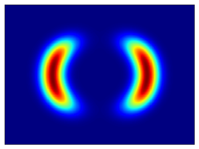
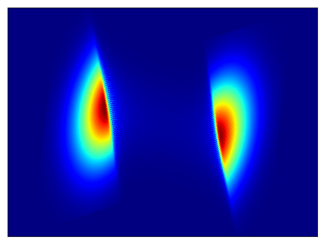
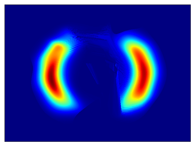
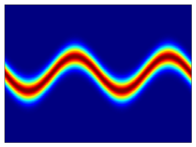
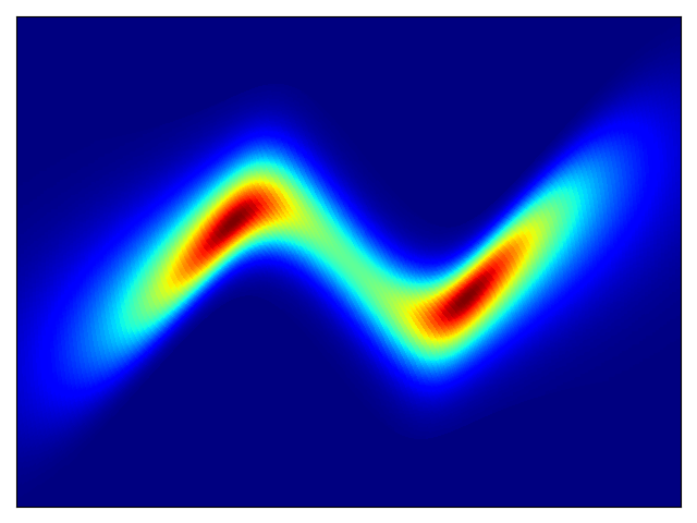
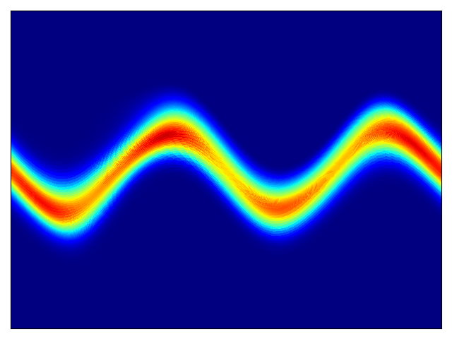
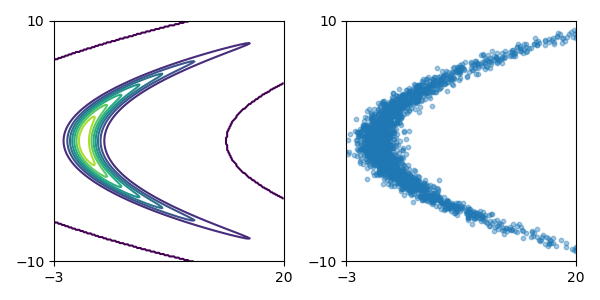
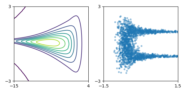
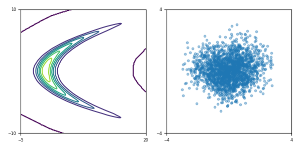
Toy density model (cf. Figure 1 in paper):

Target density	Learned density with MADE and random numbers driving MADE	Learned density with MAF 5 layers and random numbers driving MAF

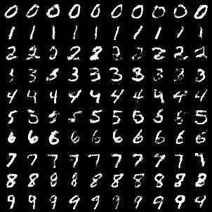
Class-conditional generated images from MNIST using MAF (5) model; generated data arrange by decreasing log probability (cf. Figure 3 in paper):

Usage

To train model:

python maf.py -- train \
              -- model=['made' | 'mademog' | 'maf' | 'mafmog' | 'realnvp'] \
              -- dataset=['POWER' | 'GAS' | 'HEPMASS' | 'MINIBOONE' | 'BSDS300' | MNIST'] \
              -- n_blocks=[for maf/mafmog and realnvp specify # of MADE-blocks / coupling layers] \
              -- n_components=[if mixture of Gaussians, specify # of components] \
              -- conditional [if MNIST, can train class-conditional log likelihood] \
              -- [add'l options see py file]

To evaluate model:

python maf.py -- evaluate \
              -- restore_file=[path to .pt checkpoint]
              -- [options of the saved model: n_blocks, n_hidden, hidden_size, n_components, conditional]

To generate data from a trained model (for MNIST dataset):

python maf.py -- generate \
              -- restore_file=[path to .pt checkpoint]
              -- dataset='MNIST'
              -- [options of the saved model: n_blocks, n_hidden, hidden_size, n_components, conditional]

Datasets

Datasets and preprocessing code are forked from the MAF authors' implementation here. The unzipped datasets should be symlinked into the ./data folder or the data_dir argument should be specified to point to the actual data.

References

The original Theano implementation by the authors https://github.com/gpapamak/maf/
https://github.com/ikostrikov/pytorch-flows

Variational inference with normalizing flows

Implementation of Variational Inference with Normalizing Flows

Results

Density estimation of 2-d test energy potentials (cf. Table 1 & Figure 3 in paper).

Target density	Flow K = 2	Flow K = 32	Training parameters
			weight init Normal(0,1), base dist. scale 2
			weight init Normal(0,1), base dist. scale 1
			weight init Normal(0,1), base dist. scale 1, weight decay 1e-3
			weight init Normal(0,1), base dist. scale 4, weight decay 1e-3

Usage

To train model:

python planar_flow.py -- train \
                      -- target_potential=[choice from u_z1 | u_z2 | u_z3 | u_z4] \
                      -- flow_length=[# of layers in flow] \
                      -- [add'l options]

Additional options are: base distribution (q0) scale, weight initialization scale, weight decay, learnable first affine layer (I did not find adding an affine layer beneficial).

To evaluate model:

python planar_flow.py -- evaluate \
                      -- restore_file=[path to .pt checkpoint]

Useful resources

casperkaae/parmesan#22

Dependencies

python 3.6
pytorch 1.0
numpy
matplotlib
tensorboardX

Some of the datasets further require:

pandas
sklearn
h5py

WonwoongCho / normalizing_flows

Normalizing flows

Block Neural Autoregressive Flow

Results

Usage

Useful resources

Glow: Generative Flow with Invertible 1x1 Convolutions

Results

Samples at varying temperatures

Samples at temperature 0.7:

Model A attribute manipulation on in-distribution sample:

Model A attribute manipulation on 'out-of-distribution' sample (i.e. me):

Usage

Datasets

References

Masked Autoregressive Flow

Results

Usage

Datasets

References

Variational inference with normalizing flows

Results

Usage

Useful resources

Dependencies

Some of the datasets further require:

About

Languages