

![]()
straintables is a tool that helps to evaluate differences
among gene loci across mutiple genomes of the same species.
This software is composed of two parts.
The first component is an in-silico version of the PCR reaction,
where regions designated as primer pairs are matched across the genomes
so the region between the primers can be retrieved.
Secondly, there is a dissimilarity matrix generator that creates matrices
based in the differences across the retrieved sequences.
straintables has different modes of operation.
The primers used to fetch genomic regions
may be user-defined or found by
brute force searches on top of the gene sequence.
These searches use
an user-provided identifier that points to a sequence
located inside an annotation file to
retrieve the desired region's boundaries.
Analysis proceeds while it counts the SNPs that diverge from the primer-bound sequences found at each genome, then builds a dissimilarity matrix for each region.
Further clustering is done, based on the DMs.
The viewer interface is simple and shows how the pairwise distances between regions from all analyzed genomes.
This package is composed by few independent python scripts which are installed as system commands. The commands are listed here.
This step is carried by the module straintables.Executable.primerFinder.
For each designated loci, the app will try to find the complement and/or the original sequence of both primers on all genomes. If both primers are found in a genome, the sequence between those primers is extracted and it proceeds to the next genome.
If every genome got its amplicon for the current locus the script saves the sequences, then goes goes to the next.
If for some reason not every genome is sucessfull with given pair of primers, the script retrieves the gene sequence from the master genome and fetch random sequences near the beginning and near the gene end, to be used as primers. This step only happens if the locus name defined by the user matches a gene name, or locus on the genome annotation. Otherwise, the locus is discarded.
Some available genomes are complement-reversed. The script will make sure that loci sequences for every genome are in the same orientation.
After getting the loci sequence from all the genomes, the visualization of the differences among genomes is done in two fronts:
- The multifasta file containing sequence for one loci among all genomes is passed through ClustalW2
- The the SNPs are detected and scored.
- One Dissimilarity Matrix is created, showing which genome groups have similar locus.
- Dissimilarity Matrices can be viewed individually as
.pdffiles,.npypython files, or grouped at the visualization toolstview.
- The primary locus multifasta file is sent to MeshClust, which will detect clusters among genome's locus. Default MeshClust identity parameters is
0.999. - The output of MeshClust is parsed at the visualization tool, which decorates genomes names at the Dissimilarity Matrix labels according to it's cluster group.
Afther the pipeline executes the docking and evaluation scripts, the user can execute stview <result_directory_path> in order to view the results.
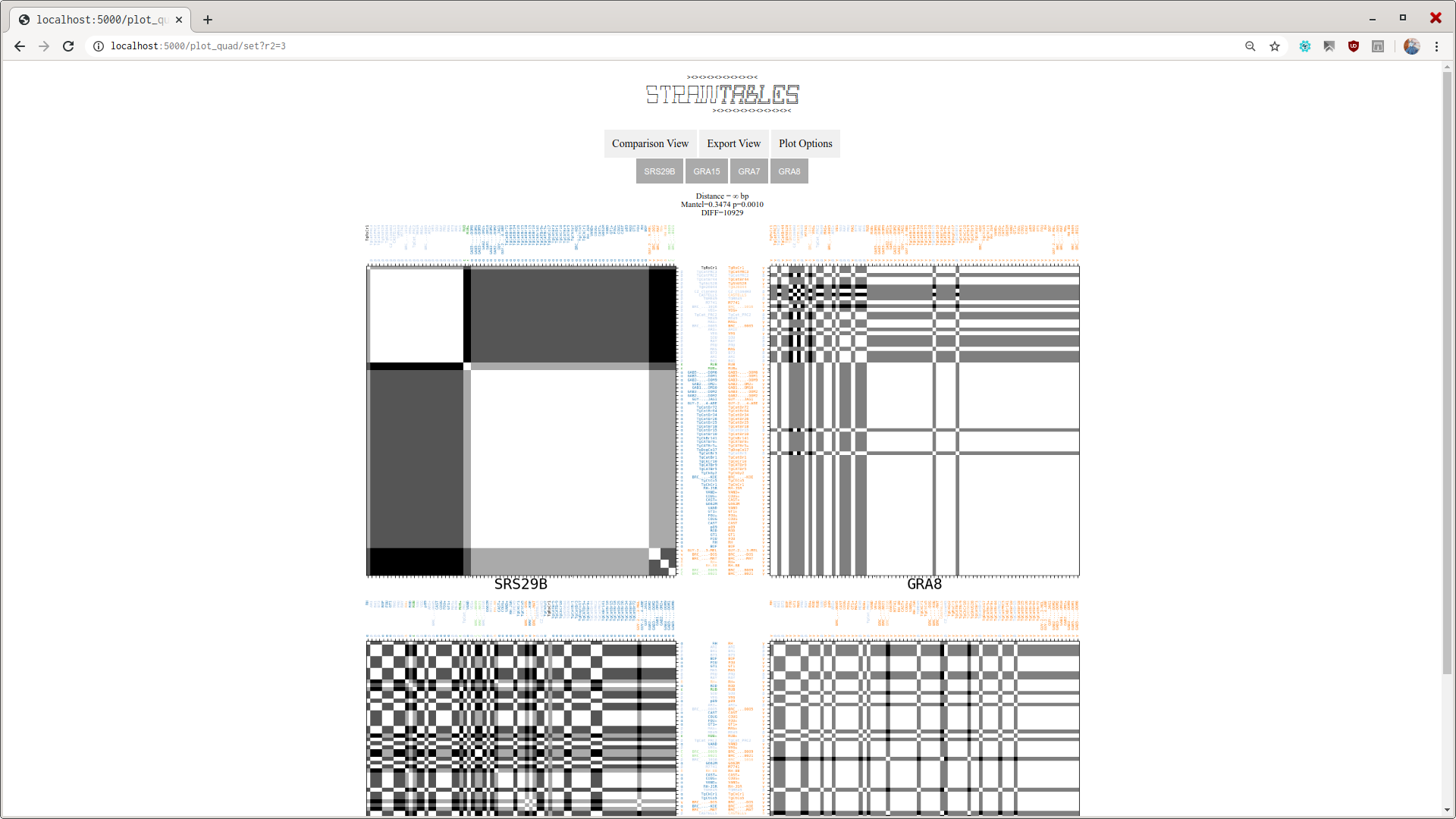
More statistical analysis on the Dissimilarity Matrices are carried, mostly using python's skbio module. The interpretation of analysis is under construction.
By looking at a pair of D. Matrices at a time, both corresponding to locus that are neighbors, the user may have an insight on data of the studied organism, like the recombination frequency.
straintables requires Python3.6+
- from pipy:
pip install setuptools numpy scipy cython --user

!! We run pip twice because the modules installed on the first step may have installation issues
!! If they fail to install, check the pip message log, it contains info for missing required system packages.


pip install straintables --user

!! Executable scripts are now at ~/.local/bin by default,
!! symlink them to your $PATH, add this folder to your $PATH,
!! or run pip without "--user" and with admin privileges, which is not recommended.
conda install -c gabzn straintables
conda update straintables
!!Then the executables should be available on conda's $PATH.
If the setup command shown above fails, there should be a problem with the build of some required python module.
Take note of which module is failing, and create a issue ticket on this repository and/or check google if it has some answer to the problem.
This has never been tested on windows, but should work. The python modules numpy, scipy, cython which should installed before straintables can raise errors on installation, and the error message should give directions to where the problem is, and they occour mostly due to missing system packages which are required by the mentioned modules.
A Dockerfile is provided as an experimental way of running this software for advanced users.
This file may also be used as reference of the required packages on Linux systems.
Here is a list of external software that are required or optional straintables' operation.
The executables should be available at your $PATH.
The alignment step of straintables requires ClustalO installed on your
system.
The recombination analysis step of straintables has MeShCluSt as an optional dependency.
Having it installed on the system will enable genome group clustering to be totally independend from the alignment software, as MeShCluSt does the clustering
on top of unaligned .fasta files.
This step will define the organism under analysis, so it's adivised run this inside a new directory, having one dir for each organism.
The following commands download each genome matching the query organism from NCBI, along with one annotation file for one specified strain.
Each of the command below will create and populate the folders genomes and annotations, so make your choice from the examples and run one of them.
To download Toxoplasma gondii genomes, strain ME49 annotation:
$stdownload --organism "Toxoplasma gondii" --strain ME49

With lactobacillus plantarum, strain WCFS1 annotation:
$stdownload --organism "Lactobacillus plantarum" --strain WCFS1

Ten genomes of Saccharomyces cerevisiae:
$stdownload --organism "Saccharomyces cerevisiae" --max 10
Although the script stdownload contatins various methods to ensure the correct file names for downloaded genomes,
it's recommended to check the folder after the process for weird names
that would otherwise be shown on the resulting matrices.
The user can manually add desired genomes and annotations, as explained in the next subsections:
- The annotation file serve as a guide for automatic primer docking, since they contain the boundaries for each locus.
- One
.gbffannotation file atannotationfolder is required.
- The genome files are the root of the analysis.
- One multifasta file per strain.
- They should be placed at the
genomesfolder.
-
Put the wanted Locus names, ForwardPrimers and ReversePrimers on a
.csvfile inside thePrimerfolder. The primer sequences are optional, leave blank to trigger the automatic primer search. Look for the examples. -
stgenomeplineis the pipeline script, it calls analysis components at proper order. -
Check the results at the result folder that is equal to the
Primerfile selected for the run. Result folders are down theAlignmentsfolder.
$ stprimer -d annotations -c X -o Primers/TEST.csv -p 0.01
$ stgenomepline -p Primers/TEST.csv
$ stview analysisResults/TEST
- Make your own primer
.csvfile, namedPrimers/chr_X.csvfor this example. It should have blank primer fields.
@file: Primers/chr_X.csv
CDPK
IMC2A
AP2X1
TGME49_227830
Then, execute:
$stgenomepline -p Primers/chr_X.csv
- Then view similarity matrices and phylogenetic trees on
pdffiles atAlignments/chr_Xfolder.
- Follow Example 2, except now the primer file can have a pair of primers designed for each loci:
- Some primers, if missing or problematic, will trigger the automatic primer search.
@file: Primers/chr_X.csv
LocusName,ForwardPrimer,ReversePrimer
CDPK1,ACAAAGGCTACTTCTACCTC,TTCTATGTGGGGATGCAGAG
IMC2A,,GACGGACGCATGGCTTGCTG
AP2X1,GCTCAAGCTGCTCCCCGGGC,TCGACGGAGGTGCTCCAACC
stdownload [--help]
stprimer [--help]
stgenomepline [--help]
stview [--help]
stprotein [--help] (under development & undocumented)
- As the pipeline unfolds, the user defined
WorkingDirectoryfolder (argument-d) will be created and populated with files of various kinds, in the order described below. It's not required to read these files manually if you stick to thestviewvisualization tool.
.fastaSequence files, one holding the amplicon found for each loci..alnAlignment files, one for each loci..aln.npyDissimilarity Matrix files, one for each loci..pdfDissimilarity Matrix Plot files, one for each loci;
- We also have some
.csvfiles with information on those regions.
-
MatchedRegions.csv: Information on matched regions, their position on each genome and more. -
AlignedRegions.csv: Information on matched regions after alignment, mostly number of snps. -
PrimerData.csv: Information on matched primers, mostly their position on each genome and orientation. -
PWMAnalysis.csv: Extended analysis on matched regions, a comparison of each pair of regions.
Some python scripts on the main module are not called within stgenomepline or stfastapline. They are optional analysis tools and should be launched by the user.
stviewThe basic one. This will launch a webserver with default addresslocalhost:5000where you can point your browser to and view the dissimilarity matrices built.
Alternatively, you can use straintables as you would use MatGAT, where you just
have a few multifasta file with many compatible short sequences, one file per region, and just
want to see dissimilarity matrices for them. The entire workflow is described below:
$stfastapline -d DIRECTORY_WITH_FASTA_FILES
$stview DIRECTORY_WITH_FASTA_FILES
The first command is a mini pipeline and should be executed only once. As of the current version, you'll need more than one region to execute this.