Time complexity
- BigO -> upper bound. O(n)
- Big omega -> lower bound. Ω(n)
- Big theta -> lower and upper bound. O(n) and Ω(n)
Amortized Time
- Average time taken per operation, if you do many operations
- If inserting N elements takes O(N) total work. Each insertion is O(1) on average, even though some insertions take O(N) time in the worst case.
Amortised time explained in simple terms:
If you do an operation say a million times, you don't really care about the worst-case or the best-case of that operation - what you care about is how much time is taken in total when you repeat the operation a million times.
So it doesn't matter if the operation is very slow once in a while, as long as "once in a while" is rare enough for the slowness to be diluted away. Essentially amortised time means "average time taken per operation, if you do many operations". Amortised time doesn't have to be constant; you can have linear and logarithmic amortised time or whatever else.
Let's take mats' example of a dynamic array, to which you repeatedly add new items. Normally adding an item takes constant time (that is, O(1)). But each time the array is full, you allocate twice as much space, copy your data into the new region, and free the old space. Assuming allocates and frees run in constant time, this enlargement process takes O(n) time where n is the current size of the array.
So each time you enlarge, you take about twice as much time as the last enlarge. But you've also waited twice as long before doing it! The cost of each enlargement can thus be "spread out" among the insertions. This means that in the long term, the total time taken for adding m items to the array is O(m), and so the amortised time (i.e. time per insertion) is O(1).
x[-1]is the last element. You can work backwards by doing x[-2], etc.list.sort()works in Python
- Stack: pop, push, peek, isEmpty (LIFO)
- Queue: add, remove, peek, isEmpty (FIFO)
- Tree construction, traversal, and manipulation algorithms.
- Binary trees, n-ary trees, and trie-trees
- You should be familiar with at least one flavor of balanced binary tree, whether it's a red/black tree, a splay tree or an AVL tree, and you should know how it's implemented.
- Three basic ways to represent a graph in memory (objects and pointers, matrix, and adjacency list), and you should familiarize yourself with each representation and its pros and cons.
- Tree traversal algorithms: BFS and DFS, and know the difference between inorder, postorder and preorder traversal (for trees).
- You should know their computational complexity, their tradeoffs, and how to implement them in real code.
- If you get a chance, study up on fancier algorithms, such as Dijkstra and A* (for graphs).
- Binary Search Tree -> all left descendants values are less than or equal to root node value. All right descendants values are greater than root node value.
- Binary Tree just means it has up to 2 children.
- Not all trees are binary trees.
- Tree with up to 3 children is a ternary tree.
- Efficiency
- Space
- Average: O(n)
- Worst: O(n)
- Search
- Average: O(log n)
- Worst: O(n)
- Insert
- Average: O(log n)
- Worst: O(n)
- Delete
- Average: O(log n)
- Worst: O(n)
- Space
- Balanced enough to ensure O(log n) times for insert and find.
- Red-Black tree or AVL tree
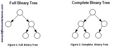
- Complete Binary Trees
- Binary tree in which every level of the tree is fully filled (maybe not the last level).
- The last level is filled, it is filled left to right.
- Full Binary Trees
- Every node has either zero or two children.
- No nodes have only one child.
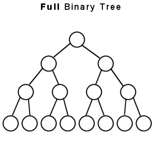
- Perfect Binary Trees
- Both full and complete.
- All leaf nodes will be at the same level, and this level has the maximum number of nodes.
- A perfect tree must have exactly
2^k - 1nodes (where k is the number of levels).
- Self-balancing binary search tree.
- Binary search tree so -> all left descendants values are less than or equal to root node value. All right descendants values are greater than root node value.
- The new principal is that it is SELF-BALANCING.
- Properties:
- Stores in each node the height of the subtree rooted at this node.
- For any node you can check if it is height balanced:
- The height of the left subtree and the height of the right subtree differ by no more than one. This presents situations where the tree gets too lopsided.
- balance(n) = n.left.height - n.right.height
- -1 <= balance(n) <= 1
- Insert:
- When you insert the balance of some nodes might change to -2 or 2. When we're unwinding the recursive stack ,we check and fix the balance at each node. We perform rotations.
- Rotations can either be left or right rotations. The right rotation is an inverse of the left rotation.
- Efficiency
- Space
- Average: O(n)
- Worst: O(n)
- Search
- Average: O(log n)
- Worst: O(log n)
- Insert
- Average: O(1)
- Worst: O(log n)
- Delete
- Average: O(1)
- Worst: O(log n)
- Space
- Rotation:
- Left Right shape: Left rotation
- Left Left shape: Right rotation
- Right Left shape: Right rotation
- Right Right shape: Left rotation
- Left or Right means: For the current node is the height of the left subtree greater or the right subtree.
- Left Left (etc.) means: For the current node is the height of the left subtree greater or the right subtree. In that subtree (Left or Right) is the height of the left subtree greater or the right subtree.
- Efficiency
- Space
- Average: O(n)
- Worst: O(n)
- Search
- Average: O(log n)
- Worst: O(log n)
- Insert
- Average: O(1)
- Worst: O(log n)
- Delete
- Average: O(1)
- Worst: O(log n)
- Space
- Splay trees maintain efficiency by reshaping the tree in response to lookups on it
- That way, frequently-accessed elements move up toward the top of the tree and have better lookup times. The shape of splay trees is not constrained, and varies based on what lookups are performed.
-
The operations to balance the trees are different, but both occur on the average in O(1) with maximum in O(log n).
-
Real difference between the two is the limiting height. For a tree of size n:
- A red-black tree's height is at most: 2*log_2(n+1)
- An AVL tree's height is strictly less than: some complex equation
-
AVL trees
- Insertion/Removal is slower. Retrieval is faster.
- AVL trees are more rigidly balanced than red-black trees, leading to slower insertion and removal but faster retrieval.
- For lookup-intensive applications, AVL trees are faster than red-black trees because they are more rigidly balanced.
-
Red Black trees
- RB-Trees guarantee O(1) rotations per insert operation.
- RB-Trees gain this advantage from conceptually being 2-3 trees without carrying around the overhead of dynamic node structures.
- Physically RB-Trees are implemented as binary trees, the red/black-flags simulate 2-3 behavior.
-
AVL trees
- One key difference between the structures is that AVL trees guarantee fast lookup (O(log n)) on each operation, while splay trees can only guarantee that any sequence of n operations takes at most O(n log n) time.
- If you need real-time lookups, the AVL tree is likely to be better.
- However, AVL trees are more useful in multithreaded environments with lots of lookups, because lookups in an AVL tree can be done in parallel while they can't in splay trees.
-
Splay trees
- Splay trees tend to be much faster on average, so if you want to minimize the total runtime of tree lookups, the splay tree is likely to be better.
- Splay trees support some operations such as splitting and merging very efficiently, while the corresponding AVL tree operations are more involved and less efficient.
- Splay trees are more memory-efficient than AVL trees, because they do not need to store balance information in the nodes.
- Because splay trees reshape themselves based on lookups, if you only need to access a small subset of the elements of the tree, or if you access some elements much more than others, the splay tree will outperform the AVL tree.
- Finally, splay trees tend to be easier to implement than AVL trees, since the rotation logic is much easier.
-
Time efficiency
- AVL tree insertion, deletion, and lookups take O(log n) time each.
- Splay trees have these same guarantees, but the guarantee is only in an amortized sense.
- Any long sequence of operations will take at most O(n log n) time, but individual operations might take as much as O(n) time.
- In-Order Traversal:
- Left
- Current node
- Right
- Pre-Order Traversal:
- Current
- Left
- Right
- Post-Order Traversal:
- Left
- Right
- Current

- Complete Binary Tree (totally filled other than the rightmost elements on the last level).
- Min heap is where each node is smaller than its children. The root is the minimum element in the tree.
- Built into Python
from heapq import heappush, heappop
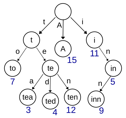
- Null nodes (* nodes) are used to indicate complete words.
- A trie can check if a string is a valid prefix in O(K) time, where K is the length of the string.
- The term trie comes from retrieval.
- A tree is a type of graph. Not all graphs are trees.
- A tree is a connected graph without cycles.
- A graph is simply a collection of nodes with edges between (some of) them.
- Can be directed or undirected.
- Graph might consist of multiple isolated subgraphs.
- If there is a path between every pair of vertices, it is called a "connected graph".
- The graph can also have cycles.
- Acyclical graph is one without cycles.
- Adjacency List
- Vertices are stored as records or objects, and every vertex stores a list of adjacent vertices.
- This data structure allows the storage of additional data on the vertices.
- Additional data can be stored if edges are also stored as objects, in which case each vertex stores its incident edges and each edge stores its incident vertices.
class Graph {
    public Node[] nodes;
}

class Node {
    public String name;
    public Node[] children;
}
- Adjacency Matrices
- A two-dimensional matrix, in which the rows represent source vertices and columns represent destination vertices.
- Data on edges and vertices must be stored externally.
- Only the cost for one edge can be stored between each pair of vertices.
- NxN boolean matrix. (N = number of nodes).
- A numerical value for
matrix[i][j]indicates an edge from node i to node j.
- Extra
- In an undirected graph, an adjacency matrix will be symmetric.
- In a directed graph, it will not (necessarily) be.
- Objects and pointers
- These are just basic data structures in Java you would represent this with classes like edges and vertices.
Vertex a = new Vertex(1);
Vertex b = new Vertex(2);
Edge edge = new Edge(a, b, 30);
- Incidence matrix (surprise forth)
- A two-dimensional Boolean matrix, in which the rows represent the vertices and columns represent the edges. The entries indicate whether the vertex at a row is incident to the edge at a column.
- A
truevalue formatrix[i][j]indicates an edge from node i to node j.
- Efficiency
- Store graph:
- Adjacency list: O(|V| + |E|)
- Adjacency matrix: O(|V|^2)
- Incidence matrix: O(|V| * |E|)
- Objects and pointers
- Add vertex:
- Adjacency list: O(1)
- Adjacency matrix: O(|V|^2)
- Incidence matrix: O(|V| * |E|)
- Objects and pointers
- Add edge:
- Adjacency list: O(1)
- Adjacency matrix: O(1)
- Incidence matrix: O(|V| * |E|)
- Objects and pointers
- Remove vertex:
- Adjacency list: O(|E|)
- Adjacency matrix: O(|V|^2)
- Incidence matrix: O(|V| * |E|)
- Objects and pointers
- Remove edge:
- Adjacency list: O(|E|)
- Adjacency matrix: O(1)
- Incidence matrix: O(|V| * |E|)
- Objects and pointers
- Query: are vertices x and y adjacent? (assuming that their storage positions are known)
- Adjacency list: O(|V|)
- Adjacency matrix: O(1)
- Incidence matrix: O(|E|)
- Objects and pointers
- Store graph:
- Remarks:
- Adjacency list:
- Slow to remove vertices and edges, because it needs to find all vertices or edges.
- Adjacency matrix:
- Slow to add or remove vertices, because matrix must be resized/copied.
- Incidence matrix:
- Slow to add or remove vertices and edges, because matrix must be resized/copied.
- Objects and pointers
- Adjacency list:
-
Adjacency list
- Adjacency lists are generally preferred because they efficiently represent sparse graphs.
-
Adjacency matrix
- Adjacency matrix is preferred if the graph is dense, that is the number of edges |E| is close to the number of vertices squared, |V|^2.
- If one must be able to quickly look up if there is an edge connecting two vertices.
-
Sparse graphs
- A graph in which the number of edges is close to the minimal number of edges.
- Sparse graph can be a disconnected graph.
-
Dense graph
- A graph in which the number of edges is close to the maximal number of edges.
- BFS
- The time complexity can be expressed as O(|V|+|E|) since every vertex and every edge will be explored in the worst case.
- |V| is the number of vertices.
- |E| is the number of edges in the graph.
- Note that O(|E|) may vary between O(1) and O(|V|^2), depending on how sparse the input graph is.
- Space complexity: O(|V|),
- The time complexity can be expressed as O(|V|+|E|) since every vertex and every edge will be explored in the worst case.
- DFS
- Worst case performance:
- O(|E|) for explicit graphs traversed without repetition. (The one we use)
- O(b^d) for implicit graphs with branching factor b searched to depth d.
- Worst case space complexity: O(|V|)
- Worst case performance:
- Implicit graphs are infinite graphs. They can't be stored in memory so they are generated as you move positions or perform some action. Basically not implicit.
- Explicit graphs are normal graphs that we store in memory and perform actions upon.
- BFS
- If you know a solution is not far from the root of the tree, a breadth first search (BFS) might be better.
- If the tree is very deep and solutions are rare, depth first search (DFS) might take an extremely long time, but BFS could be faster.
- If the tree is very wide, a BFS might need too much memory, so it might be completely impractical.
- If solutions are frequent but located deep in the tree, BFS could be impractical.
- DFS
- If the search tree is very deep you will need to restrict the search depth for depth first search (DFS), anyway (for example with iterative deepening).
- DFS has much lower memory requirements than BFS.
- From What I understand iterative deepening does DFS down to depth 1 then does DFS down to depth of 2 ... down to depth n , and so on till it finds no more levels.
- You cache the previous levels.
- In computer science, Iterative deepening depth-first search (IDDFS) is a state space search strategy in which a depth-limited search is run repeatedly, increasing the depth limit with each iteration until it reaches d, the depth of the shallowest goal state.
- IDDFS is equivalent to breadth-first search, but uses much less memory; on each iteration, it visits the nodes in the search tree in the same order as depth-first search, but the cumulative order in which nodes are first visited is effectively breadth-first.
- BFS
- Finding the shortest path between two nodes u and v
- Serialization/Deserialization of a binary tree vs serialization in sorted order, allows the tree to be re-constructed in an efficient manner.
- DFS
- Finding connected components.
- Topological sorting.
- Dijkstra's Algorithm
- Edge with weights
- Shortest path between two points in a weighted directed graph (which might have cycles).
- All edges must have positive values.
- Algorithm
- Start off at s
- For each s's outbound edges, clone ourselves and start walking. If the edge (s, x) has weight 5, we should actually take 5 minutes to get there.
- Each time we get to a node, check if anyone's been there before. If so, then just stop. We're automatically not as fast as another path since someone beat us here from s. If no one has been here before, then clone ourselves and head out in all possible directions.
- The first one to get to t wins.
- Uses:
path_weight[node]previous[node]remaining: minimum priority queue.
- Implementation (p 635):
- Lots of edges then v^2 will be close to e. Then you can use priority queue with an array. Total runtime is O(v^2).
- Sparse graph: e is much less than v^2. Min-heap implementation is better. Total runtime is O((v + 2) log v).
- Dijkstra’s shortest path algorithm is very fairly intuitive:
- Initialize the passed nodes with the source and current shortest path with zero.
- Include the node that minimize the current shortest path plus the edge distance among all edges whose tail are in the passed nodes and head in uncharted nodes.
- Update the current shortest path and repeat step 2 until all nodes are passed.
- A*
- Topological Sort
- In computing, a hash table (hash map) is a data structure used to implement an associative array, a structure that can map keys to values.
- A hash table uses a hash function to compute an index into an array of buckets or slots, from which the desired value can be found.
- Most famous classes of NP-complete problems, such as traveling salesman and the knapsack problem.
- Traveling salesman
TravellingSaleman(Path: sequence of points) {
   Compute the initial length of Path
   loop {
      for each pair of points U,V, calculate the change to the length
             caused by swapping U and V;
      choose the pair U,V
           that causes the largest decrease in the length of Path
      if no pair of points causes any decrease,
          then return Path;
      swap U and V in Path and decrement the length by the change
    }
}
- You should be able to solve a problem recursively, and know how to use and repurpose common recursive algorithms to solve new problems.
- Conversely, you should be able to take a given algorithm and prove inductively that it will do what you claim it will do.
int fibonacci(int i) {
    if (i == 0) return 0;
    if (i == 1) return 1;
    return fibonacci(i - 1) + fibonacci(i - 2);
}
- Some interviewers ask basic discrete math questions. This is more prevalent at Google than at other companies because we are surrounded by counting problems, probability problems, and other Discrete Math 101 situations.
- Spend some time before the interview on the essentials of combinatorics and probability. You should be familiar with n-choose-k problems and their ilk – the more the better.
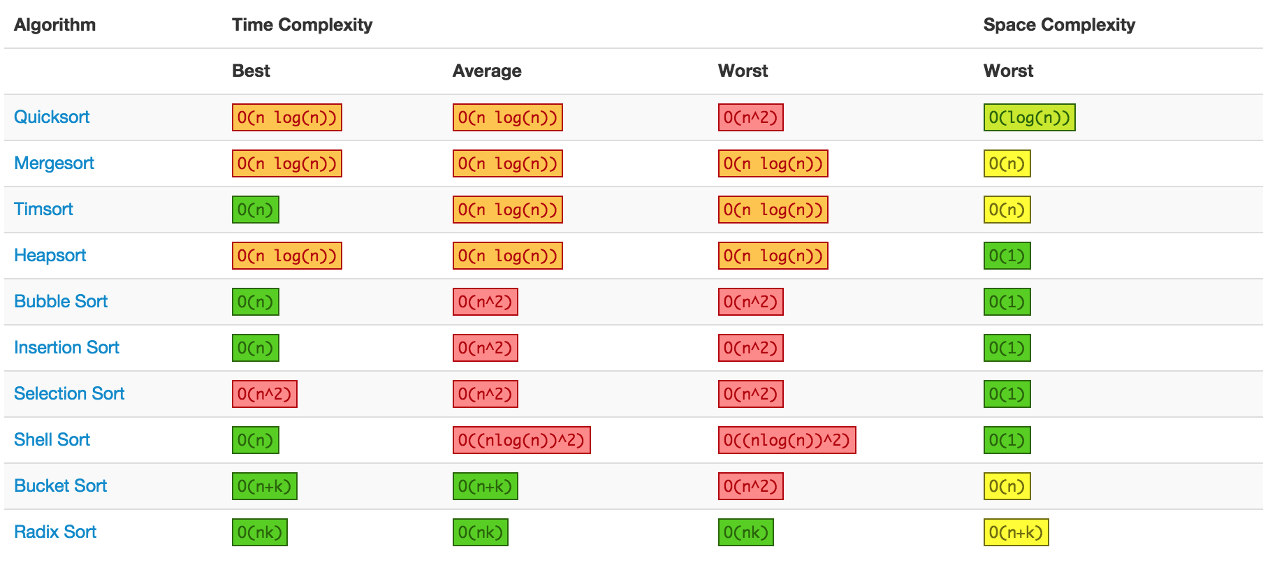
- Time complexity
- Average O(n log n)
- Worst: O(n^2)
- Memory
- Average: O(log n)
- Pick a random element and partition the array, such that all numbers that are less than the partitioning element come before all elements that are greater than it.
- Repeatedly partition the array it will eventually become sorted.
- Uses divide and conquer to recursively divide and sort the list
- Time Complexity: O(n log n)
- Space Complexity: O(n) Auxiliary (due to the auxiliary space used to merge parts of the array)
- Merge method operates by copying all the elements from the target array segment into a helper array. Keeps track of where the start of the left and right halves should be.